Archive for the ‘OpenGL’ Category
Homage to Structure Synth
This post is a follow-up to something I wrote exactly one year ago: Mesh Generation with Python.
In the old post, I discussed a number of ways to generate 3D shapes in Python, and I posted some OpenGL screenshots to show off the geometry.
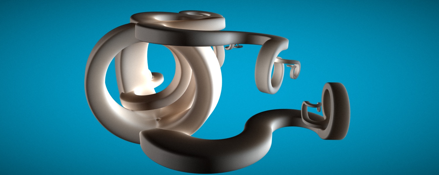
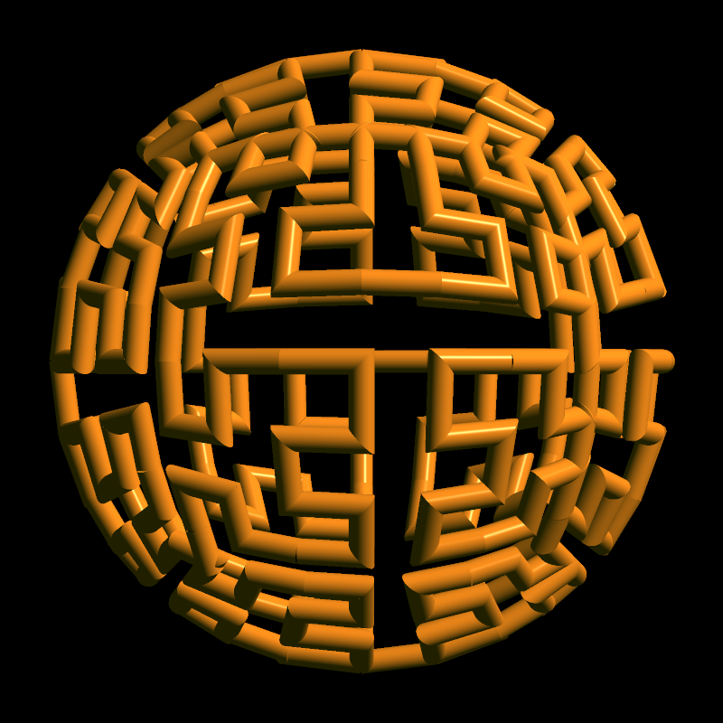
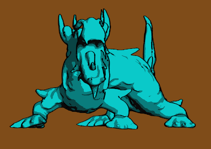
Since this is my first post since joining Pixar, I figured it would be fun to use RenderMan rather than OpenGL to show off some new procedurally-generated shapes. Sure, my new images don’t render at interactive rates, but they’re nice and high-quality:

Beautiful Lindenmayer Systems
My favorite L-system from Mikael Hvidtfeldt Christensen is his Nouveau Variation; when I first saw it, I stared at it for half an hour; it’s hypnotically mathematical and surreal. He generates his art using his own software, Structure Synth.
To make similar creations without the help of Mikael’s software, I use the same XML format and Python script that I showed off in my 2010 post (here), with an extension to switch from one rule to another when a particular rule’s maximum depth is reached.
The other improvement I made was in the implementation itself; rather than using recursion to evaluate the L-system rules, I use a Python list as a stack. This turned out to simplify the code.
Here’s the XML representation of Mikael’s beautiful “Nouveau” L-system, which I used to generate all the images on this page:
<rules max_depth="1000">
    <rule name="entry">
        <call count="16" transforms="rz 20" rule="hbox"/>
    </rule>
    <rule name="hbox"><call rule="r"/></rule>
    <rule name="r"><call rule="forward"/></rule>
    <rule name="r"><call rule="turn"/></rule>
    <rule name="r"><call rule="turn2"/></rule>
    <rule name="r"><call rule="turn4"/></rule>
    <rule name="r"><call rule="turn3"/></rule>
    <rule name="forward" max_depth="90" successor="r">
        <call rule="dbox"/>
        <call transforms="rz 2 tx 0.1 sa 0.996" rule="forward"/>
    </rule>
    <rule name="turn" max_depth="90" successor="r">
        <call rule="dbox"/>
        <call transforms="rz 2 tx 0.1 sa 0.996" rule="turn"/>
    </rule>
    <rule name="turn2" max_depth="90" successor="r">
        <call rule="dbox"/>
        <call transforms="rz -2 tx 0.1 sa 0.996" rule="turn2"/>
    </rule>
    <rule name="turn3" max_depth="90" successor="r">
        <call rule="dbox"/>
        <call transforms="ry -2 tx 0.1 sa 0.996" rule="turn3"/>
    </rule>
    <rule name="turn4" max_depth="90" successor="r">
        <call rule="dbox"/>
        <call transforms="ry -2 tx 0.1 sa 0.996" rule="turn4"/>
    </rule>
    <rule name="turn5" max_depth="90" successor="r">
        <call rule="dbox"/>
        <call transforms="rx -2 tx 0.1 sa 0.996" rule="turn5"/>
    </rule>
    <rule name="turn6" max_depth="90" successor="r">
        <call rule="dbox"/>
        <call transforms="rx -2 tx 0.1 sa 0.996" rule="turn6"/>
    </rule>
    <rule name="dbox">
        <instance transforms="s 2.0 2.0 1.25" shape="boxy"/>
    </rule>
</rules>
Python Snippets for RenderMan
RenderMan lets you assign names to gprims, which I find useful when it reports errors. RenderMan also lets you assign gprims to various “ray groups”, which is nice when you’re using AO or Global Illumination; it lets you include/exclude certain geometry from ray-casts.
Given these two labels (an identifier and a ray group), I found it useful to extend RenderMan’s Python binding with a utility function:
def SetLabel( self, label, groups = '' ):
    """Sets the id and ray group(s) for subsequent gprims"""
    self.Attribute(self.IDENTIFIER,{self.NAME:label})
    if groups != '':
        self.Attribute("grouping",{"membership":groups})
Since Python lets you dynamically add methods to a class, you can graft the above function onto the Ri class like so:
prman.Ri.SetLabel = SetLabel
ri = prman.Ri()
# do some init stuff....
ri.SetLabel("MyHeroShape", "MovingGroup")
# instance a gprim...
I also found it useful to write some Python functions that simply called out to external processes, like the RSL compiler and the brickmap utility:
def CompileShader(shader):
    """Compiles the given RSL file"""
    print 'Compiling %s...' % shader
    retval = os.system("shader %s.sl" % shader)
    if retval:
        quit()

def CreateBrickmap(base):
    """Creates a brick map from a point cloud"""
    if os.path.exists('%s.bkm' % base):
        print "Found brickmap for %s" % base
    else:
        print "Creating brickmap for %s..." % base
        if not os.path.exists('%s.ptc' % base):
            print "Error: %s.ptc has not been generated." % base
        else:
            os.system("brickmake %s.ptc %s.bkm" % (base, base))
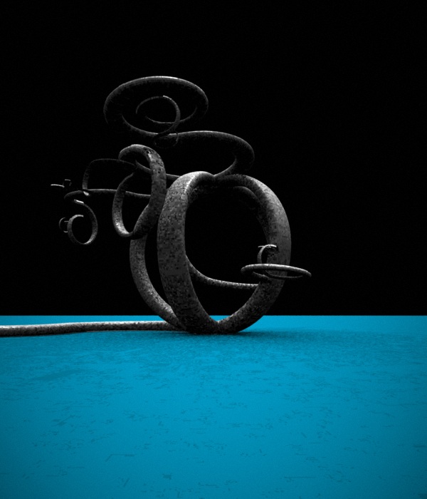
Here’s another image of the same L-system, using a different random seed:

Reminds me of Salvadore Dalí…
Some RSL Fun
The RenderMan stuff was fairly straightforward. I’m using a bog-standard AO shader:
class ComputeOcclusion(string hitgroup = "";
                       color em = (1,0,1);
                       float samples = 64)
{
  public void surface(output color Ci, Oi)
  {
    normal Nn = normalize(N);
    float occ = occlusion(P, Nn, samples,
                          "maxdist", 100.0,
                          "subset", hitgroup);

    Ci = (1 - occ) * Cs * Os;
    Ci *= em;
    Oi = Os;
  }
}
Hurray, that was my first RSL code snippet on the blog! I’m also using an imager shader to achieve the same vignette effect that Mikael used for his artwork. It just applies a radial dimming operation and adds a bit of noise to give it a photographic look:
class Vignette()
{
   public void imager(output varying color Ci; output varying color Oi)
   {
        float x = s - 0.5;
        float y = t - 0.5;
        float d = x * x + y * y;
        Ci *= 1.0 - d;

        float n = (cellnoise(s*1000, t*1000) - 0.5);
        Ci += n * 0.025;
   }
}
Downloads
Here are my Python scripts and RSL code for your enjoyment:
Gallery


Deep Opacity Maps
In the video, the light source is slowly spinning around the smoke stack, showing that a deep opacity map is generated at every frame. For now it’s being computed rather inefficiently, by performing a full raycast over each voxel in the light map. Here’s my fragment shader for generating the opacity map:
in float gLayer;
out float FragColor;

uniform sampler3D Density;
uniform vec3 LightPosition = vec3(1.0, 1.0, 2.0);
uniform float LightIntensity = 10.0;
uniform float Absorption = 10.0;
uniform float LightStep;
uniform int LightSamples;
uniform vec3 InverseSize;

void main()
{
    vec3 pos = InverseSize * vec3(gl_FragCoord.xy, gLayer);
    vec3 lightDir = normalize(LightPosition-pos) * LightStep;
    float Tl = 1.0;
    vec3 lpos = pos + lightDir;

    for (int s = 0; s < LightSamples; ++s) {
        float ld = texture(Density, pos).x;
        Tl *= 1.0 - Absorption * LightStep * ld;
        if (Tl <= 0.01)
            break;

        // Would be faster if this conditional is replaced with a tighter loop
        if (lpos.x < 0 || lpos.y < 0 || lpos.z < 0 ||
            lpos.x > 1 || lpos.y > 1 || lpos.z > 1)
            break;

        lpos += lightDir;
    }

    float Li = LightIntensity*Tl;
    FragColor = Li;
}
It would be much more efficient to align the light volume with the light direction, allowing you to remove the loop and accumulate results from the previous layer. Normally you can’t sample from the same texture that you’re rendering to, but in this case it would be a different layer of the FBO, so it would be legal.
Another potential optimization is using MRT with 8 render targets, and packing 4 depths into each layer; this would generate 32 layers per instance rather than just one!
Here’s another video just for fun, taken with a higher resolution grid. It doesn’t run at interactive rates (I forced the video to 30 fps) but the crepuscular shadow rays sure look cool:
Noise-Based Particles, Part II
In Part I, I covered Bridson’s “curl noise” method for particle advection, describing how to build a static grid of velocity vectors. I portrayed the construction process as an acyclic image processing graph, where the inputs are volumetric representations of obstacles and turbulence.
The demo code in Part I was a bit lame, since it moved particles on the CPU. In this post, I show how to perform advection on the GPU using GL_TRANSFORM_FEEDBACK. For more complex particle management, I’d probably opt for OpenCL/CUDA, but for something this simple, transform feedback is the easiest route to take.
Initialization
In my particle simulation, the number of particles remains fairly constant, so I decided to keep it simple by ping-ponging two staticly-sized VBOs. The beauty of transform feedback is that the two VBOs can stay in dedicated graphics memory; no bus travel.
In the days before transform feedback (and CUDA), the only way to achieve GPU-based advection was sneaky usage of the fragment shader and a one-dimensional FBO. Those days are long gone — OpenGL now allows you to effectively shut off the rasterizer, performing advection completely in the vertex shader and/or geometry shader.
The first step is creating the two ping-pong VBOs, which is done like you’d expect:
GLuint ParticleBufferA, ParticleBufferB;
const int ParticleCount = 100000;
ParticlePod seed_particles[ParticleCount] = { ... };

// Create VBO for input on even-numbered frames and output on odd-numbered frames:
glGenBuffers(1, &ParticleBufferA);
glBindBuffer(GL_ARRAY_BUFFER, ParticleBufferA);
glBufferData(GL_ARRAY_BUFFER, sizeof(seed_particles), &seed_particles[0], GL_STREAM_DRAW);
glBindBuffer(GL_ARRAY_BUFFER, 0);

// Create VBO for output on even-numbered frames and input on odd-numbered frames:
glGenBuffers(1, &ParticleBufferB);
glBindBuffer(GL_ARRAY_BUFFER, ParticleBufferB);
glBufferData(GL_ARRAY_BUFFER, sizeof(seed_particles), 0, GL_STREAM_DRAW);
glBindBuffer(GL_ARRAY_BUFFER, 0);
Note that I provided some initial seed data in ParticleBufferA, but I left ParticleBufferB uninitialized. This initial seeding is the only CPU-GPU transfer in the demo.
By the way, I don’t think the GL_STREAM_DRAW hint really matters; most drivers are smart enough to manage memory in a way that they think is best.
The only other initialization task is binding the outputs from the vertex shader (or geometry shader). Watch out because this needs to take place after you compile the shaders, but before you link them:
GLuint programHandle = glCreateProgram();

GLuint vsHandle = glCreateShader(GL_VERTEX_SHADER);
glShaderSource(vsHandle, 1, &vsSource, 0);
glCompileShader(vsHandle);
glAttachShader(programHandle, vsHandle);

const char* varyings[3] = { "vPosition", "vBirthTime", "vVelocity" };
glTransformFeedbackVaryings(programHandle, 3, varyings, GL_INTERLEAVED_ATTRIBS);

glLinkProgram(programHandle);
Yep, that’s a OpenGL program object that only has a vertex shader attached; no fragment shader!
I realize it smells suspiciously like Hungarian, but I like to prefix my vertex shader outputs with a lowercase “v”, geometry shader outputs with lowercase “g”, etc. It helps me avoid naming collisions when trickling a value through the entire pipe.
Advection Shader
The vertex shader for noise-based advection is crazy simple. I stole the randhash function from a Robert Bridson demo; it was surprisingly easy to port to GLSL.
-- Vertex Shader

in vec3 Position;
in float BirthTime;
in vec3 Velocity;

out vec3 vPosition;
out float vBirthTime;
out vec3 vVelocity;

uniform sampler3D Sampler;
uniform vec3 Size;
uniform vec3 Extent;
uniform float Time;
uniform float TimeStep = 5.0;
uniform float InitialBand = 0.1;
uniform float SeedRadius = 0.25;
uniform float PlumeCeiling = 3.0;
uniform float PlumeBase = -3;

const float TwoPi = 6.28318530718;
const float InverseMaxInt = 1.0 / 4294967295.0;

float randhash(uint seed, float b)
{
    uint i=(seed^12345391u)*2654435769u;
    i^=(i<<6u)^(i>>26u);
    i*=2654435769u;
    i+=(i<<5u)^(i>>12u);
    return float(b * i) * InverseMaxInt;
}

vec3 SampleVelocity(vec3 p)
{
    vec3 tc;
    tc.x = (p.x + Extent.x) / (2 * Extent.x);
    tc.y = (p.y + Extent.y) / (2 * Extent.y);
    tc.z = (p.z + Extent.z) / (2 * Extent.z);
    return texture(Sampler, tc).xyz;
}

void main()
{
    vPosition = Position;
    vBirthTime = BirthTime;

    // Seed a new particle as soon as an old one dies:
    if (BirthTime == 0.0 || Position.y > PlumeCeiling) {
        uint seed = uint(Time * 1000.0) + uint(gl_VertexID);
        float theta = randhashf(seed++, TwoPi);
        float r = randhashf(seed++, SeedRadius);
        float y = randhashf(seed++, InitialBand);
        vPosition.x = r * cos(theta);
        vPosition.y = PlumeBase + y;
        vPosition.z = r * sin(theta);
        vBirthTime = Time;
    }

    // Advance the particle using an additional half-step to reduce numerical issues:
    vVelocity = SampleVelocity(Position);
    vec3 midx = Position + 0.5f * TimeStep * vVelocity;
    vVelocity = SampleVelocity(midx);
    vPosition += TimeStep * vVelocity;
}
Note the sneaky usage of gl_VertexID to help randomize the seed. Cool eh?
Using Transform Feedback
Now let’s see how to apply the above shader from your application code. You’ll need to use three functions that you might not be familiar with: glBindBufferBase specifies the target VBO, and gl{Begin/End}TransformFeedback delimits the draw call that performs advection. I’ve highlighted these calls below, along with the new enable that allows you to turn off rasterization:
// Set up the advection shader:
glUseProgram(ParticleAdvectProgram);
glUniform1f(ParticleAdvectProgram, timeLoc, currentTime);

// Specify the source buffer:
glEnable(GL_RASTERIZER_DISCARD);
glBindBuffer(GL_ARRAY_BUFFER, ParticleBufferA);
glEnableVertexAttribArray(SlotPosition);
glEnableVertexAttribArray(SlotBirthTime);
char* pOffset = 0;
glVertexAttribPointer(SlotPosition, 3, GL_FLOAT, GL_FALSE, 16, pOffset);
glVertexAttribPointer(SlotBirthTime, 1, GL_FLOAT, GL_FALSE, 16, 12 + pOffset);

// Specify the target buffer:
glBindBufferBase(GL_TRANSFORM_FEEDBACK_BUFFER, 0, ParticleBufferB);

// Perform GPU advection:
glBeginTransformFeedback(GL_POINTS);
glBindTexture(GL_TEXTURE_3D, VelocityTexture.Handle);
glDrawArrays(GL_POINTS, 0, ParticleCount);
glEndTransformFeedback();

// Swap the A and B buffers for ping-ponging, then turn the rasterizer back on:
std::swap(ParticleBufferA, ParticleBufferB);
glDisable(GL_RASTERIZER_DISCARD);
The last step is actually rendering the post-transformed particles:
glUseProgram(ParticleRenderProgram);
glBindBuffer(GL_ARRAY_BUFFER, ParticleBufferA);
glVertexAttribPointer(SlotPosition, 3, GL_FLOAT, GL_FALSE, 16, pOffset);
glVertexAttribPointer(SlotBirthTime, 1, GL_FLOAT, GL_FALSE, 16, 12 + pOffset);
glDrawArrays(GL_POINTS, 0, ParticleCount);
In my case, rendering the particles was definitely the bottleneck; the advection was insanely fast. As covered in Part I, I use the geometry shader to extrude points into view-aligned billboards that get stretched according to the velocity vector. An interesting extension to this approach would be to keep a short history (3 or 4 positions) with each particle, allowing nice particle trails, also known as “particle traces”. This brings back memories of the ASCII snake games of my youth (does anyone remember QBasic Nibbles?)
Well, that’s about it! Please realize that I’ve only covered the simplest possible usage of transform feedback. OpenGL 4.0 introduced much richer functionality, allowing you to intermingle several VBOs in any way you like, and executing draw calls without any knowledge of buffer size. If you want to learn more, check out this nice write-up from Christophe Riccio, where he describes the evolution of transform feedback:
http://www.g-truc.net/post-0269.html
Downloads
The first time you run my demo, it’ll take a while to initialize because it needs to construct the velocity field. On subsequent runs, it loads the data from an external file, so it starts up quickly. Note that I’m using the CPU to generate the velocity field; performing it on the GPU would be much, much faster.
I’ve tested the code with Visual Studio 2010. It uses CMake for the build system.
The code is released under the unlicense license.
3D Eulerian Grid
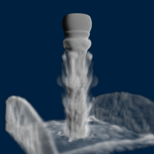
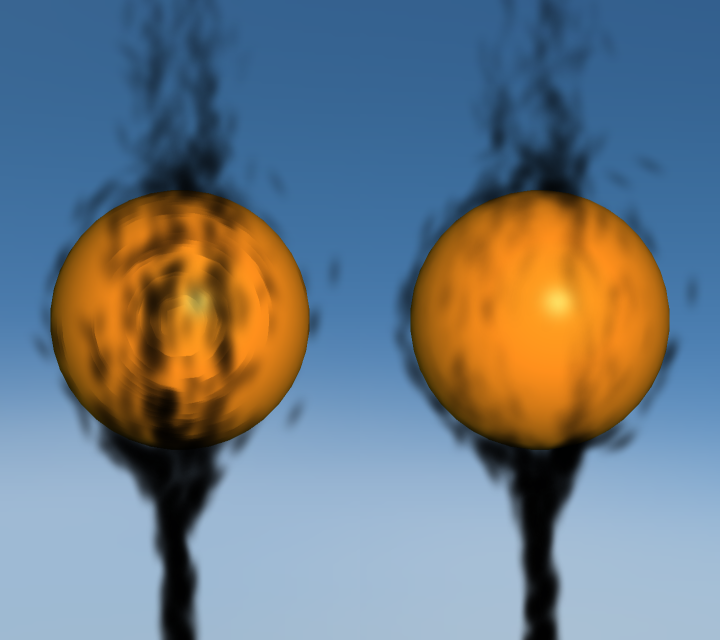
I finally extended my OpenGL-based Eulerian fluid simulation to 3D. It’s not as pretty as Miles Macklin’s stuff (here), but at least it runs at interactive rates on my GeForce GTS 450, which isn’t exactly top-of-the-line. My original blog entry, “Simple Fluid Simulation”, goes into much more detail than this post.
I thought it would be fun to invert buoyancy and gravity to make it look more like liquid nitrogen than smoke. The source code can be downloaded at the end of this post.
Extending to three dimensions was fairly straightforward. I’m still using a half-float format for my velocity texture, but I’ve obviously made it 3D and changed its format to GL_RGB16F (previously it was GL_RG16F).
The volumetric image processing is achieved by ping-ponging layered FBOs, using instanced rendering to update all slices of a volume with a single draw call and a tiny 4-vert VBO, like this:
glDrawArraysInstanced(GL_TRIANGLE_STRIP, 0, 4, numLayers);
Here are the vertex and geometry shaders that I use to make this work:
-- Vertex Shader

in vec4 Position;
out int vInstance;

void main()
{
    gl_Position = Position;
    vInstance = gl_InstanceID;
}

-- Geometry Shader

layout(triangles) in;
layout(triangle_strip, max_vertices = 3) out;

in int vInstance[3];
out float gLayer;

uniform float InverseSize;

void main()
{
    gl_Layer = vInstance[0];
    gLayer = float(gl_Layer) + 0.5;
    gl_Position = gl_in[0].gl_Position;
    EmitVertex();
    gl_Position = gl_in[1].gl_Position;
    EmitVertex();
    gl_Position = gl_in[2].gl_Position;
    EmitVertex();
    EndPrimitive();
}
Note that I offset the layer by 0.5. I’m too lazy to pass the entire texture coordinate to the fragment shader, so my fragment shader uses a gl_FragCoord trick to get to the right texture coordinate:
-- Fragment Shader

uniform vec3 InverseSize;
uniform sampler3D VelocityTexture;

void main()
{
    vec3 tc = InverseSize * vec3(gl_FragCoord.xy, gLayer);
    vec3 velocity = texture(VelocityTexture, tc).xyz;
    // ...
}
Since the fragment shader gets evaluated at pixel centers, I needed the 0.5 offset on the layer coordinate to prevent the fluid from “drifting” along the Z axis.
The fragment shaders are otherwise pretty damn similar to their 2D counterparts. As an example, I’ll show you how I extended the SubtractGradient shader, which computes the gradient vector for pressure. Previously it did something like this:
float N = texelFetchOffset(Pressure, T, 0, ivec2(0, 1)).r;
float S = texelFetchOffset(Pressure, T, 0, ivec2(0, -1)).r;
float E = texelFetchOffset(Pressure, T, 0, ivec2(1, 0)).r;
float W = texelFetchOffset(Pressure, T, 0, ivec2(-1, 0)).r;
vec2 oldVelocity = texelFetch(Velocity, T, 0).xy;
vec2 gradient = vec2(E - W, N - S) * GradientScale;
vec2 newVelocity = oldVelocity - gradient;
The new code does something like this:
float N = texelFetchOffset(Pressure, T, 0, ivec3(0, 1, 0)).r;
float S = texelFetchOffset(Pressure, T, 0, ivec3(0, -1, 0)).r;
float E = texelFetchOffset(Pressure, T, 0, ivec3(1, 0, 0)).r;
float W = texelFetchOffset(Pressure, T, 0, ivec3(-1, 0, 0)).r;
float U = texelFetchOffset(Pressure, T, 0, ivec3(0, 0, 1)).r;
float D = texelFetchOffset(Pressure, T, 0, ivec3(0, 0, -1)).r;
vec3 oldVelocity = texelFetch(Velocity, T, 0).xyz;
vec3 gradient = vec3(E - W, N - S, U - D) * GradientScale;
vec3 newVelocity = oldVelocity - gradient;
Simple!
Downloads
I’ve tested the code with Visual Studio 2010. It uses CMake for the build system. If you have trouble building it or running it, let me warn you that you need a decent graphics card and decent OpenGL drivers.
I consider this code to be on the public domain. Enjoy!
Single-Pass Raycasting
Raycasting over a volume requires start and stop points for your rays. The traditional method for computing these intervals is to draw a cube (with perspective) into two surfaces: one surface has front faces, the other has back faces. By using a fragment shader that writes object-space XYZ into the RGB channels, you get intervals. Your final pass is the actual raycast.
In the original incarnation of this post, I proposed making it into a single pass process by dilating a back-facing triangle from the cube and performing perspective-correct interpolation math in the fragment shader. Simon Green pointed out that this was a bit silly, since I can simply do a ray-cube intersection. So I rewrote this post, showing how to correlate a field-of-view angle (typically used to generate an OpenGL projection matrix) and focal length (typically used to determine ray direction). This might be useful to you if you need to integrate a raycast volume into an existing 3D scene that uses traditional rendering.
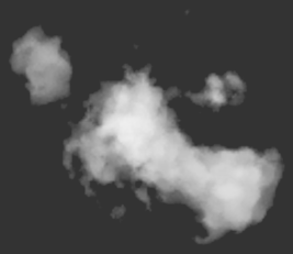
To have something interesting to render in the demo code (download is at the end of the post), I generated a pyroclastic cloud as described in this amazing PDF on volumetric methods from the 2010 SIGGRAPH course. Miles Macklin has a simply great blog entry about it here.
Recap of Two-Pass Raycasting
Here’s a depiction of the usual offscreen surfaces for ray intervals:
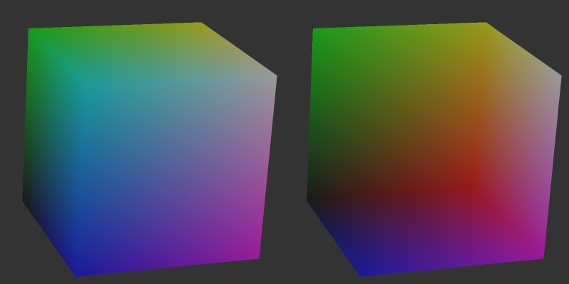
Front faces give you the start points and the back faces give you the end points. The usual procedure goes like this:
-
Draw a cube’s front faces into surface A and back faces into surface B. This determines ray intervals.
- Attach two textures to the current FBO to render to both surfaces simultaneously.
- Use a fragment shader that writes out normalized object-space coordinates to the RGB channels.
-
Draw a full-screen quad to perform the raycast.
- Bind three textures: the two interval surfaces, and the 3D texture you’re raycasting against.
- Sample the two interval surfaces to obtain ray start and stop points. If they’re equal, issue a discard.
Making it Single-Pass
To make this a one-pass process and remove two texture lookups from the fragment shader, we can use a procedure like this:
-
Draw a cube’s front-faces to perform the raycast.
- On the CPU, compute the eye position in object space and send it down as a uniform.
- Also on the CPU, compute a focal length based on the field-of-view that you’re using to generate your scene’s projection matrix.
- At the top of the fragment shader, perform a ray-cube intersection.
Raycasting on front-faces instead of a full-screen quad allows you to avoid the need to test for intersection failure. Traditional raycasting shaders issue a discard if there’s no intersection with the view volume, but since we’re guaranteed to hit the viewing volume, so there’s no need.
Without further ado, here’s my fragment shader using modern GLSL syntax:
out vec4 FragColor;

uniform mat4 Modelview;
uniform float FocalLength;
uniform vec2 WindowSize;
uniform vec3 RayOrigin;

struct Ray {
    vec3 Origin;
    vec3 Dir;
};

struct AABB {
    vec3 Min;
    vec3 Max;
};

bool IntersectBox(Ray r, AABB aabb, out float t0, out float t1)
{
    vec3 invR = 1.0 / r.Dir;
    vec3 tbot = invR * (aabb.Min-r.Origin);
    vec3 ttop = invR * (aabb.Max-r.Origin);
    vec3 tmin = min(ttop, tbot);
    vec3 tmax = max(ttop, tbot);
    vec2 t = max(tmin.xx, tmin.yz);
    t0 = max(t.x, t.y);
    t = min(tmax.xx, tmax.yz);
    t1 = min(t.x, t.y);
    return t0 <= t1;
}

void main()
{
    vec3 rayDirection;
    rayDirection.xy = 2.0 * gl_FragCoord.xy / WindowSize - 1.0;
    rayDirection.z = -FocalLength;
    rayDirection = (vec4(rayDirection, 0) * Modelview).xyz;

    Ray eye = Ray( RayOrigin, normalize(rayDirection) );
    AABB aabb = AABB(vec3(-1.0), vec3(+1.0));

    float tnear, tfar;
    IntersectBox(eye, aabb, tnear, tfar);
    if (tnear < 0.0) tnear = 0.0;

    vec3 rayStart = eye.Origin + eye.Dir * tnear;
    vec3 rayStop = eye.Origin + eye.Dir * tfar;

    // Transform from object space to texture coordinate space:
    rayStart = 0.5 * (rayStart + 1.0);
    rayStop = 0.5 * (rayStop + 1.0);

    // Perform the ray marching:
    vec3 pos = rayStart;
    vec3 step = normalize(rayStop-rayStart) * stepSize;
    float travel = distance(rayStop, rayStart);
    for (int i=0; i < MaxSamples && travel > 0.0; ++i, pos += step, travel -= stepSize) {

        // ...lighting and absorption stuff here...

    }
The shader works by using gl_FragCoord and a given FocalLength value to generate a ray direction. Just like a traditional CPU-based raytracer, the appropriate analogy is to imagine holding a square piece of chicken wire in front of you, tracing rays from your eyes through the holes in the mesh.
If you’re integrating the raycast volume into an existing scene, computing FocalLength and RayOrigin can be a little tricky, but it shouldn’t be too difficult. Here’s a little sketch I made:
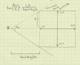
In days of yore, most OpenGL programmers would use the gluPerspective function to compute a projection matrix, although nowadays you’re probably using whatever vector math library you happen to be using. My personal favorite is the simple C++ vector library from Sony that’s included in Bullet. Anyway, you’re probably calling a function that takes a field-of-view angle as an argument:
Matrix4 Perspective(float fovy, float aspectRatio, float nearPlane, float farPlane);
Based on the above diagram, converting the fov value into a focal length is easy:
float focalLength = 1.0f / tan(FieldOfView / 2);
You’re also probably calling function kinda like gluLookAt to compute your view matrix:
Matrix4 LookAt(Point3 eyePosition, Point3 targetPosition, Vector3 up);
To compute a ray origin, transform the eye position from world space into object space, relative to the viewing cube.
Downloads
I’ve tested the code with Visual Studio 2010. It uses CMake for the build system.
I consider this code to be on the public domain. Enjoy!
Noise-Based Particles, Part I
Robert Bridson, that esteemed guru of fluid simulation, wrote a short-n-sweet 2007 SIGGRAPH paper on using Perlin noise to create turbulent effects in a divergence-free velocity field (PDF). Divergence-free means that the velocity field conforms to the incompressibility aspect of Navier-Stokes, making it somewhat believable from a physics standpoint. It’s a nice way to fake a fluid if you don’t have enough horsepower for a more rigorous physically-based system, such as the Eulerian grid in my Simple Fluid Simulation post.
The basic idea is to introduce noise into a “potential field”, then derive velocity from the potential field using the curl operator. Here’s an expansion of the curl operator that shows how to obtain 3D velocity from potential:
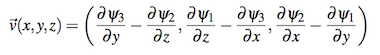
The fact that we call it “potential” and that we’re using a Ψ symbol isn’t really important. The point is to use whatever crazy values we want for our potential field and not to worry about it. As long as we keep the potential smooth (no discontinuities), it’s legal. That’s because we’re taking its curl to obtain velocity, and the curl of any smooth field is always divergence-free:

Implementation

You really only need four ingredients for this recipe:
- Distance field for the rigid obstacles in your scene
- Intensity map representing areas where you’d like to inject turbulence
- vec3-to-vec3 function for turbulent noise (gets multiplied by the above map)
- Simple, smooth field of vectors for starting potential (e.g., buoyancy)
For the third bullet, a nice-looking result can be obtained by summing up three octaves of Perlin noise. For GPU-based particles, it can be represented with a 3D RGB texture. Technically the noise should be time-varying (an array of 3D textures), but in practice a single frame of noise seems good enough.
The fourth bullet is a bit tricky because the concept of “inverse curl” is dodgy; given a velocity field, you cannot recover a unique potential field from it. Luckily, for smoke, we simply need global upward velocities for buoyancy, and coming up with a reasonable source potential isn’t difficult. Conceptually, it helps to think of topo lines in the potential field as streamlines.
The final potential field is created by blending together the above four ingredients in a reasonable manner. I created an interactive diagram with graphviz that shows how the ingredients come together. If your browser supports SVG, you can click on the diagram, then click any node to see a visualization of the plane at Z=0.

If you’re storing the final velocity field in a 3D texture, most of the processing in the diagram needs to occur only once, at startup. The final velocity field can be static as long as your obstacles don’t move.
Obtaining velocity from the potential field is done with the curl operator; in pseudocode it looks like this:
Vector3 ComputeCurl(Point3 p)
{
    const float e = 1e-4f;
    Vector3 dx(e, 0, 0);
    Vector3 dy(0, e, 0);
    Vector3 dz(0, 0, e);

    float x = SamplePotential(p + dy).z - SamplePotential(p - dy).z
            - SamplePotential(p + dz).y + SamplePotential(p - dz).y;

    float y = SamplePotential(p + dz).x - SamplePotential(p - dz).x
            - SamplePotential(p + dx).z + SamplePotential(p - dx).z;

    float z = SamplePotential(p + dx).y - SamplePotential(p - dx).y
            - SamplePotential(p + dy).x + SamplePotential(p - dy).x;

    return Vector3(x, y, z) / (2*e);
}
Equally useful is a ComputeGradient function, which is used against the distance field to obtain a value that can be mixed into the potential field:
Vector3 ComputeGradient(Point3 p)
{
    const float e = 0.01f;
    Vector3 dx(e, 0, 0);
    Vector3 dy(0, e, 0);
    Vector3 dz(0, 0, e);

    float d =    SampleDistance(p);
    float dfdx = SampleDistance(p + dx) - d;
    float dfdy = SampleDistance(p + dy) - d;
    float dfdz = SampleDistance(p + dz) - d;

    return normalize(Vector3(dfdx, dfdy, dfdz));
}
Blending the distance gradient into an existing potential field can be a bit tricky; here’s one way of doing it:
// Returns a modified potential vector, respecting the boundaries defined by distanceGradient
Vector3 BlendVectors(Vector3 potential, Vector3 distanceGradient, float alpha)
{
    float dp = dot(potential, distanceGradient);
    return alpha * potential + (1-alpha) * dp * distanceGradient;
}
The alpha parameter in the above snippet can be computed by applying a ramp function to the current distance value.
Motion Blur
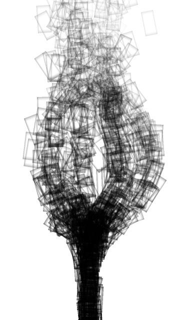
Let’s turn now to some of the rendering issues involved. Let’s assume you’ve got very little horsepower, or you’re working in a very small time slice — this might be why you’re using a noise-based solution anyway. You might only be capable of a one-thousand particle system instead of a one-million particle system. For your particles to be space-filling, consider adding some motion blur.
Motion blur might seem overkill at first, but since it inflates your billboards in an intelligent way, you can have fewer particles in your system. The image to the right (click to enlarge) shows how billboards can be stretched and oriented according to their velocities.
Note that it can be tricky to perform velocity alignment and still allow for certain viewing angles. For more on the subject (and some code), see this section of my previous blog entry.
Soft Particles
Another rendering issue that can crop up are hard edges. This occurs when you’re depth-testing billboards against obstacles in your scene — the effect is shown on the left in the image below.
Turns out that an excellent chapter in GPU Gems 3 discusses this issue. (Here’s a link to the online version of the chapter.) The basic idea is to fade alpha in your fragment shader according to the Z distance between the current fragment and the depth obstacle. This method is called soft particles, and you can see the result on the right in the comparison image.
I found that using a linear fade-out can cause particles to appear too light. To alleviate this, I decided to apply a quartic falloff to the alpha value. This makes the particle stay opaque longer with rapid fall-off. When I’m prototyping simple functions like this, I like to use Wolfram Alpha as my web-based graphing calculator . Here’s one possibility (click to view in Wolfram Alpha):
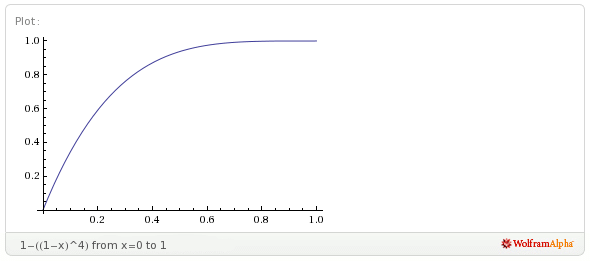
It’s tempting to use trig functions when designing ramp functions like this, but keep in mind that they can be quite costly.
Without further ado, here’s the fragment shader that I used to render my smoke particles:
uniform vec4 Color;
uniform vec2 InverseSize;
varying float gAlpha;
varying vec2 gTexCoord;
uniform sampler2D SpriteSampler;
uniform sampler2D DepthSampler;

void main()
{
    vec2 tc = gl_FragCoord.xy * InverseSize;
    float depth = texture2D(DepthSampler, tc).r;
    if (depth < gl_FragCoord.z)
        discard;

    float d = depth - gl_FragCoord.z;
    float softness = 1.0 - min(1.0, 40.0 * d);
    softness *= softness;
    softness = 1.0 - softness * softness;

    float A = gAlpha * texture2D(SpriteSampler, gTexCoord).a;
    gl_FragColor = Color * vec4(1, 1, 1, A * softness);
}
There are actually three alpha values involved in the above snippet: alpha due to the particle’s lifetime (gAlpha), alpha due to the circular nature of the sprite (SpriteSampler), and alpha due to the proximity of the nearest depth boundary (softness).
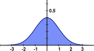
If you’d like, you can avoid the SpriteSampler lookup by evaluating the Gaussian function in the shader; I took that approach in my previous blog entry.
Next up is the compositing fragment shader that I used to blend the particle billboards against the scene. When this shader is active, the app is drawing a full-screen quad.
varying vec2 vTexCoord;
uniform sampler2D BackgroundSampler;
uniform sampler2D ParticlesSampler;

void main()
{
    vec4 dest = texture2D(BackgroundSampler, vTexCoord);
    vec4 src = texture2D(ParticlesSampler, vTexCoord);
    gl_FragColor.rgb = src.rgb * a + dest.rgb * (1.0 - a);
    gl_FragColor.a = 1.0;
}
Here’s the blending function I use when drawing the particles:
glBlendFuncSeparate(GL_SRC_ALPHA, GL_ONE_MINUS_SRC_ALPHA, GL_ZERO, GL_ONE_MINUS_SRC_ALPHA);
The rationale for this is explained in the GPU gems chapter that I already mentioned.
Streamlines
Adding a streamline renderer to your app makes it easy to visualize turbulent effects. As seen in the video to the right, it’s also pretty fun to watch the streamlines grow. The easiest way to do this? Simply use very small billboards and remove the call to glClear! Well, you’ll probably still want to clear the surface at startup time, to prevent junk. Easy peasy!
Downloads
I’ve tested the code with Mac OS X and Windows with Visual Studio 2010. It uses CMake for the build system.
I consider this code to be on the public domain. Enjoy!
Tron, Volumetric Lines, and Meshless Tubes
With Tron: Legacy hitting theaters, I thought it’d be fun to write a post on volumetric line strips. They come in handy for a variety of effects (lightsabers, lightning, particle traces, etc.). In many cases, you can render volumetric lines by drawing thin lines into an offscreen surface, then blurring the entire surface. However, in some cases, screen-space blur won’t work out for you. Maybe you’re fill-rate bound, or maybe you need immediate depth-testing. You’d prefer a single-pass solution, and you want your volumetric lines to look great even when the lines are aligned to the viewing direction.
Geometry shaders to the rescue! By having the geometry shader emit a cuboid for each line segment, the fragment shader can perform a variety of effects within the screen-space region defined by the projected cuboid. This includes Gaussian splatting, alpha texturing, or even simple raytracing of cylinders or capsules. I stole the general idea from Sébastien Hillaire.
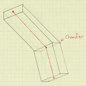
You can apply this technique to line strip primitives with or without adjacency. If you include adjacency, your geometry shader can chamfer the ends of the cuboid, turning the cuboid into a general prismoid and creating a tighter screen-space region.
I hate bloating vertex buffers with adjacency information. However, with GL_LINE_STRIP_ADJACENCY, adjacency incurs very little cost: simply add an extra vert to the beginning and end of your vertex buffer and you’re done! For more on adjacency, see my post on silhouettes or this interesting post on avoiding adjacency for terrain silhouettes.
For line strips, you might want to use GL_MAX blending rather than simple additive blending. This makes it easy to avoid extra glow at the joints.
Here’s a simplified version of the geometry shader, using old-school GLSL syntax to make Apple fans happy:
uniform mat4 ModelviewProjection;
varying in vec3 vPosition[4]; // Four inputs since we're using GL_LINE_STRIP_ADJACENCY
varying in vec3 vNormal[4];   // Orientation vectors are necessary for consistent alignment
vec4 prismoid[8]; // Scratch space for the eight corners of the prismoid

void emit(int a, int b, int c, int d)
{
    gl_Position = prismoid[a]; EmitVertex();
    gl_Position = prismoid[b]; EmitVertex();
    gl_Position = prismoid[c]; EmitVertex();
    gl_Position = prismoid[d]; EmitVertex();
    EndPrimitive();
}

void main()
{
    // Compute orientation vectors for the two connecting faces:
    vec3 p0, p1, p2, p3;
    p0 = vPosition[0]; p1 = vPosition[1];
    p2 = vPosition[2]; p3 = vPosition[3];
    vec3 n0 = normalize(p1-p0);
    vec3 n1 = normalize(p2-p1);
    vec3 n2 = normalize(p3-p2);
    vec3 u = normalize(n0+n1);
    vec3 v = normalize(n1+n2);

    // Declare scratch variables for basis vectors:
    vec3 i,j,k; float r = Radius;

    // Compute face 1 of 2:
    j = u; i = vNormal[1]; k = cross(i, j); i *= r; k *= r;
    prismoid[0] = ModelviewProjection * vec4(p1 + i + k, 1);
    prismoid[1] = ModelviewProjection * vec4(p1 + i - k, 1);
    prismoid[2] = ModelviewProjection * vec4(p1 - i - k, 1);
    prismoid[3] = ModelviewProjection * vec4(p1 - i + k, 1);

    // Compute face 2 of 2:
    j = v; i = vNormal[2]; k = cross(i, j); i *= r; k *= r;
    prismoid[4] = ModelviewProjection * vec4(p2 + i + k, 1);
    prismoid[5] = ModelviewProjection * vec4(p2 + i - k, 1);
    prismoid[6] = ModelviewProjection * vec4(p2 - i - k, 1);
    prismoid[7] = ModelviewProjection * vec4(p2 - i + k, 1);

    // Emit the six faces of the prismoid:
    emit(0,1,3,2); emit(5,4,6,7);
    emit(4,5,0,1); emit(3,2,7,6);
    emit(0,3,4,7); emit(2,1,6,5);
}
Glow With Point-Line Distance

Here’s my fragment shader for Tron-like glow. For this to link properly, the geometry shader needs to output some screen-space coordinates for the nodes in the line strip (gEndpoints[2] and gPosition). The fragment shader simply computes a point-line distance, using the result for the pixel’s intensity. It’s actually computing distance as “point-to-segment” rather than “point-to-infinite-line”. If you prefer the latter, you might be able to make an optimization by moving the distance computation up into the geometry shader.
uniform vec4 Color;

varying vec2 gEndpoints[2];
varying vec2 gPosition;

uniform float Radius;
uniform mat4 Projection;

// Return distance from point 'p' to line segment 'a b':
float line_distance(vec2 p, vec2 a, vec2 b)
{
    float dist = distance(a,b);
    vec2 v = normalize(b-a);
    float t = dot(v,p-a);
    vec2 spinePoint;
    if (t > dist) spinePoint = b;
    else if (t > 0.0) spinePoint = a + t*v;
    else spinePoint = a;
    return distance(p,spinePoint);
}

void main()
{
    float d = line_distance(gPosition, gEndpoints[0], gEndpoints[1]);
    gl_FragColor = vec4(vec3(1.0 - 12.0 * d), 1.0);
}
Raytraced Cylindrical Imposters
I’m not sure how useful this is, but you can actually go a step further and perform a ray-cylinder intersection test in your fragment shader and use the surface normal to perform lighting. The result: triangle-free tubes! By writing to the gl_FragDepth variable, you can enable depth-testing, and your tubes integrate into the scene like magic; no tessellation required. Here’s an excerpt from my fragment shader. (For the full shader, download the source code at the end of the article.)
vec3 perp(vec3 v)
{
    vec3 b = cross(v, vec3(0, 0, 1));
    if (dot(b, b) < 0.01)
        b = cross(v, vec3(0, 1, 0));
    return b;
}

bool IntersectCylinder(vec3 origin, vec3 dir, out float t)
{
    vec3 A = gEndpoints[1]; vec3 B = gEndpoints[2];
    float Epsilon = 0.0000001;
    float extent = distance(A, B);
    vec3 W = (B - A) / extent;
    vec3 U = perp(W);
    vec3 V = cross(U, W);
    U = normalize(cross(V, W));
    V = normalize(V);
    float rSqr = Radius*Radius;
    vec3 diff = origin - 0.5 * (A + B);
    mat3 basis = mat3(U, V, W);
    vec3 P = diff * basis;
    float dz = dot(W, dir);
    if (abs(dz) >= 1.0 - Epsilon) {
        float radialSqrDist = rSqr - P.x*P.x - P.y*P.y;
        if (radialSqrDist < 0.0)
            return false;
        t = (dz > 0.0 ? -P.z : P.z) + extent * 0.5;
        return true;
    }

    vec3 D = vec3(dot(U, dir), dot(V, dir), dz);
    float a0 = P.x*P.x + P.y*P.y - rSqr;
    float a1 = P.x*D.x + P.y*D.y;
    float a2 = D.x*D.x + D.y*D.y;
    float discr = a1*a1 - a0*a2;
    if (discr < 0.0)
        return false;

    if (discr > Epsilon) {
        float root = sqrt(discr);
        float inv = 1.0/a2;
        t = (-a1 + root)*inv;
        return true;
    }

    t = -a1/a2;
    return true;
}
Motion-Blurred Billboards

Emitting cuboids from the geometry shader are great fun, but they’re overkill for many tasks. If you want to render short particle traces, it’s easier just to emit a quad from your geometry shader. The quad can be oriented and stretched according to the screen-space projection of the particle’s velocity vector. The tricky part is handling degenerate conditions: velocity might be close to zero, or velocity might be Z-aligned.
One technique to deal with this is to interpolate the emitted quad between a vertically-aligned square and a velocity-aligned rectangle, and basing the lerping factor on the magnitude of the velocity vector projected into screen-space.
Here’s the full geometry shader and fragment shader for motion-blurred particles. The geometry shader receives two endpoints of a line segment as input, and uses these to determine velocity.
-- Geometry Shader

varying in vec3 vPosition[2];
varying out vec2 gCoord;

uniform mat4 ModelviewProjection;
uniform float Radius;
uniform mat3 Modelview;
uniform mat4 Projection;
uniform float Time;

float Epsilon = 0.001;

void main()
{
    vec3 p = mix(vPosition[0], vPosition[1], Time);
    float w = Radius * 0.5;
    float h = w * 2.0;
    vec3 u = Modelview * (vPosition[1] - vPosition[0]);

    // Determine 't', which represents Z-aligned magnitude.
    // By default, t = 0.0.
    // If velocity aligns with Z, increase t towards 1.0.
    // If total speed is negligible, increase t towards 1.0.
    float t = 0.0;
    float nz = abs(normalize(u).z);
    if (nz > 1.0 - Epsilon)
        t = (nz - (1.0 - Epsilon)) / Epsilon;
    else if (dot(u,u) < Epsilon)
        t = (Epsilon - dot(u,u)) / Epsilon;

    // Compute screen-space velocity:
    u.z = 0.0;
    u = normalize(u);

    // Lerp the orientation vector if screen-space velocity is negligible:
    u = normalize(mix(u, vec3(1,0,0), t));
    h = mix(h, w, t);

    // Compute the change-of-basis matrix for the billboard:
    vec3 v = vec3(-u.y, u.x, 0);
    vec3 a = u * Modelview;
    vec3 b = v * Modelview;
    vec3 c = cross(a, b);
    mat3 basis = mat3(a, b, c);

    // Compute the four offset vectors:
    vec3 N = basis * vec3(0,w,0);
    vec3 S = basis * vec3(0,-w,0);
    vec3 E = basis * vec3(-h,0,0);
    vec3 W = basis * vec3(h,0,0);

    // Emit the quad:
    gCoord = vec2(1,1); gl_Position = ModelviewProjection * vec4(p+N+E,1); EmitVertex();
    gCoord = vec2(-1,1); gl_Position = ModelviewProjection * vec4(p+N+W,1); EmitVertex();
    gCoord = vec2(1,-1); gl_Position = ModelviewProjection * vec4(p+S+E,1); EmitVertex();
    gCoord = vec2(-1,-1); gl_Position = ModelviewProjection * vec4(p+S+W,1); EmitVertex();
    EndPrimitive();
}

-- Fragment Shader

varying vec2 gCoord;

void main()
{
    float r2 = dot(gCoord, gCoord);
    float d = exp(r2 * -1.2); // Gaussian Splat
    gl_FragColor = vec4(vec3(d), 1.0);
}
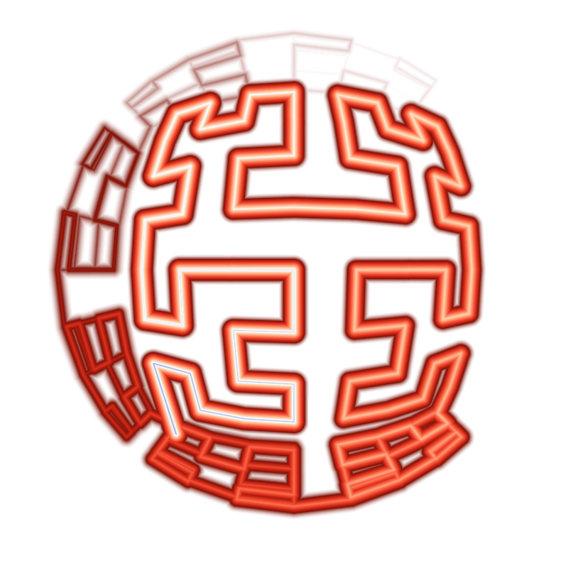
Diversion: Hilbert Cubed Sphere
You might’ve noticed the interesting path that I’ve used for my examples. This is a Hilbert curve drawn on the surface of a cube, with the cube deformed into a sphere. If you think of a Hilbert curve as a parametric function from R1 to R2, then any two points that are reasonably close in R1 are also reasonably close in R2. Cool huh? Here’s some C++ code for how I constructed the vertex buffer for the Hilbert cube:
struct Turtle {
    void Move(float dx, float dy, bool changeFace = false) {
        if (changeFace) ++Face;
        switch (Face) {
            case 0: P += Vector3(dx, dy, 0); break;
            case 1: P += Vector3(0, dy, dx); break;
            case 2: P += Vector3(-dy, 0, dx); break;
            case 3: P += Vector3(0, -dy, dx); break;
            case 4: P += Vector3(dy, 0, dx); break;
            case 5: P += Vector3(dy, dx, 0); break;
        }
        HilbertPath.push_back(P);
    }
    Point3 P;
    int Face;
};

static void HilbertU(int level)
{
    if (level == 0) return;
    HilbertD(level-1);      HilbertTurtle.Move(0, -dist);
    HilbertU(level-1);      HilbertTurtle.Move(dist, 0);
    HilbertU(level-1);      HilbertTurtle.Move(0, dist);
    HilbertC(level-1);
}

static void HilbertD(int level)
{
    if (level == 0) return;
    HilbertU(level-1);      HilbertTurtle.Move(dist, 0);
    HilbertD(level-1);      HilbertTurtle.Move(0, -dist);
    HilbertD(level-1);      HilbertTurtle.Move(-dist, 0);
    HilbertA(level-1);
}

static void HilbertC(int level)
{
    if (level == 0) return;
    HilbertA(level-1);      HilbertTurtle.Move(-dist, 0);
    HilbertC(level-1);      HilbertTurtle.Move(0, dist);
    HilbertC(level-1);      HilbertTurtle.Move(dist, 0);
    HilbertU(level-1);
}

static void HilbertA(int level)
{
    if (level == 0) return;
    HilbertC(level-1);      HilbertTurtle.Move(0, dist);
    HilbertA(level-1);      HilbertTurtle.Move(-dist, 0);
    HilbertA(level-1);      HilbertTurtle.Move(0, -dist);
    HilbertD(level-1);
}

void CreateHilbertCube(int lod)
{
    HilbertU(lod); HilbertTurtle.Move(dist, 0, true);
    HilbertU(lod); HilbertTurtle.Move(0, dist, true);
    HilbertC(lod); HilbertTurtle.Move(0, dist, true);
    HilbertC(lod); HilbertTurtle.Move(0, dist, true);
    HilbertC(lod); HilbertTurtle.Move(dist, 0, true);
    HilbertD(lod);
}
Deforming the cube into a sphere is easy: just normalize the positions!
Downloads
I tested the code on Mac OS X and on Windows. It uses CMake for the build system, and I consider the code to be on the public domain. A video of the app is embedded at the bottom of this page. Enjoy!
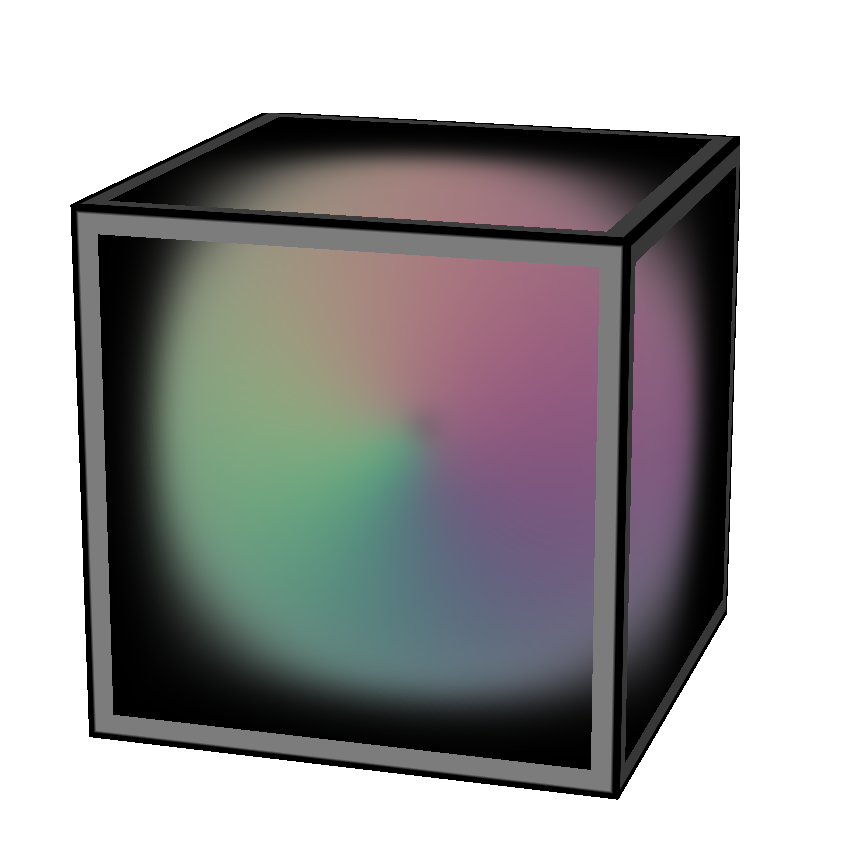
Volumetric Splatting
Instanced rendering turns out to be useful for volumetric graphics. I first came across the concept in this excellent chapter in GPU Gems 3, which briefly mentions that instancing can voxelize a model in only 1 draw call using nothing but a quad. After reading this, I had the idea of using instancing to efficiently render volumetric splats. Splatting is useful for creating distance fields and Voronoi maps. It can also be used to extrude a streamline into a space-filling velocity field.
In this article, I show how volumetric splatting can be implemented efficiently with instancing. I show how to leverage splatting to extrude a circular streamline into a toroidal field of velocity vectors. This technique would allow an artist to design a large velocity field (e.g., for a particle system), simply by specifying a small animation path through space. My article also covers some basics of modern-day volume rendering on the GPU.
Volume Raycasting
Before I show you my raycasting shader, let me show you a neat trick to easily obtain the start and stop points for the rays. It works by drawing a cube into a pair of floating-point RGB surfaces, using a fragment shader that writes out object-space coordinates. Frontfaces go into one color attachment, backfaces in the other. This results in a tidy set of start/stop positions. Here are the shaders:
-- Vertex

in vec4 Position;
out vec3 vPosition;
uniform mat4 ModelviewProjection;

void main()
{
    gl_Position = ModelviewProjection * Position;
    vPosition = Position.xyz;
}

-- Fragment

in vec3 vPosition;
out vec3 FragData[2];

void main()
{
    if (gl_FrontFacing) {
        FragData[0] = 0.5 * (vPosition + 1.0);
        FragData[1] = vec3(0);
    } else {
        FragData[0] = vec3(0);
        FragData[1] = 0.5 * (vPosition + 1.0);
    }
}
Update: I recently realized that the pair of endpoint surfaces can be avoided by performing a quick ray-cube intersection in the fragment shader. I wrote a blog entry about it here.
You’ll want to first clear the surfaces to black, and enable simple additive blending for this to work correctly. Note that we’re using multiple render targets (MRT) to generate both surfaces in a single pass. To pull this off, you’ll need to bind a FBO that has two color attachments, then issue a glDrawBuffers command before rendering, like this:
GLenum renderTargets[2] = {GL_COLOR_ATTACHMENT0, GL_COLOR_ATTACHMENT1};
glDrawBuffers(2, &renderTargets[0]);
// Render cube...
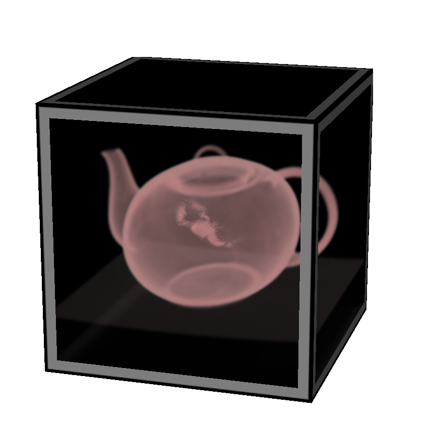
The next step is the actual raycasting, which is done by drawing a fullscreen quad with a longish fragment shader. We need to set up three texture samplers: two for the start/stop surfaces and one for the 3D volume texture itself. The following fragment shader performs raycasts against a single-channel 3D texture, which I used to generate the teapot image to the right. I obtained the scorpion-in-teapot volume data from this site at the University of Tübingen.
uniform sampler2D RayStart;
uniform sampler2D RayStop;
uniform sampler3D Volume;

out vec4 FragColor;
in vec3 vPosition;

uniform float StepLength = 0.01;

void main()
{
    vec2 coord = 0.5 * (vPosition.xy + 1.0);
    vec3 rayStart = texture(RayStart, coord).xyz;
    vec3 rayStop = texture(RayStop, coord).xyz;

    if (rayStart == rayStop) {
        discard;
        return;
    }

    vec3 ray = rayStop - rayStart;
    float rayLength = length(ray);
    vec3 stepVector = StepLength * ray/rayLength;

    vec3 pos = rayStart;
    vec4 dst = vec4(0);
    while (dst.a < 1 && rayLength > 0) {
        float density = texture(Volume, pos).x;
        vec4 src = vec4(density);
        src.rgb *= src.a;
        dst = (1.0 - dst.a) * src + dst;
        pos += stepVector;
        rayLength -= StepLength;
    }

    FragColor = dst;
}
Note the front-to-back blending equation inside the while loop; Benjamin Supnik has a good article about front-to-back blending on his blog. One advantage of front-to-back raycasting: it allows you to break out of the loop on fully-opaque voxels.
Volumetric Lighting
You’ll often want to create a more traditional lighting effect in your raycaster. For this, you’ll need to obtain surface normals somehow. Since we’re dealing with volume data, this might seem non-trivial, but it’s actually pretty simple.
Really there are two problems to solve: (1) detecting voxels that intersect surfaces in the volume data, and (2) computing the normal vectors at those positions. Turns out both of these problems can be addressed with an essential concept from vector calculus: the gradient vector points in the direction of greatest change, and its magnitude represents the amount of change. If we can compute the gradient at a particular location, we can check its magnitude to see if we’re crossing a surface. And, conveniently enough, the direction of the gradient is exactly what we want to use for our lighting normal!
The gradient vector is made up of the partial derivatives along the three axes; it can be approximated like this:
vec3 ComputeGradient(vec3 P)
{
    float L = StepLength;
    float E = texture(VolumeSampler, P + vec3(L,0,0));
    float N = texture(VolumeSampler, P + vec3(0,L,0));
    float U = texture(VolumeSampler, P + vec3(0,0,L));
    return vec3(E - V, N - V, U - V);
}
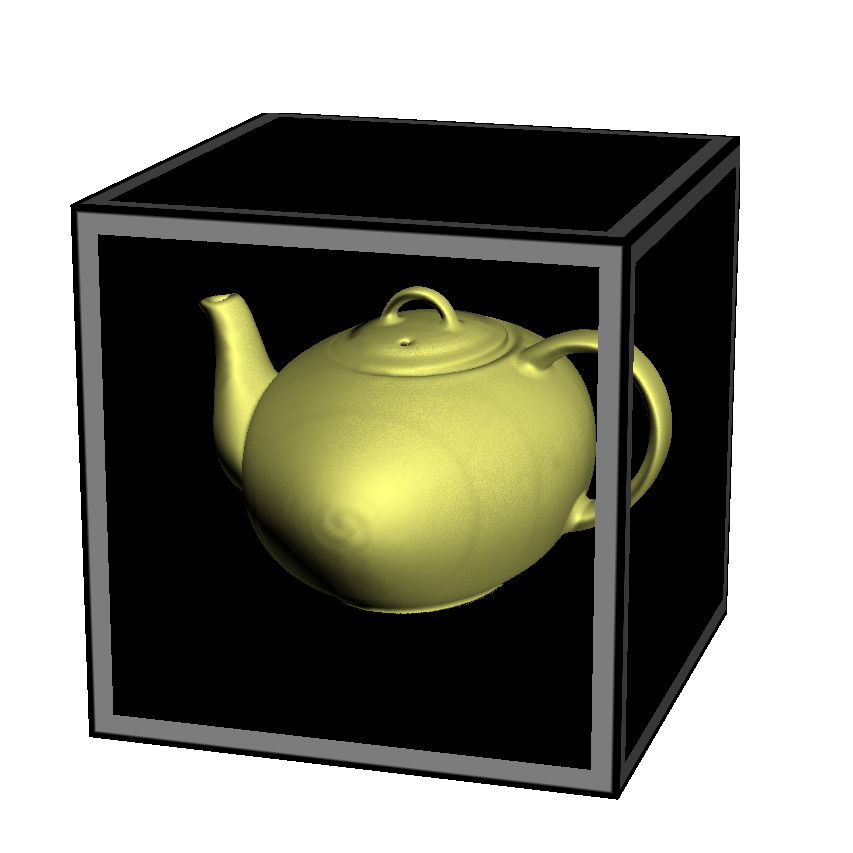
For the teapot data, we’ll compute the gradient for lighting normals only when the current voxel’s value is above a certain threshold. This lets us avoid making too many texture lookups. The shader looks like this:
out vec4 FragColor;
in vec3 vPosition;

uniform sampler2D RayStart;
uniform sampler2D RayStop;
uniform sampler3D Volume;

uniform float StepLength = 0.01;
uniform float Threshold = 0.45;

uniform vec3 LightPosition;
uniform vec3 DiffuseMaterial;
uniform mat4 Modelview;
uniform mat3 NormalMatrix;

float lookup(vec3 coord)
{
    return texture(Volume, coord).x;
}

void main()
{
    vec2 coord = 0.5 * (vPosition.xy + 1.0);
    vec3 rayStart = texture(RayStart, coord).xyz;
    vec3 rayStop = texture(RayStop, coord).xyz;

    if (rayStart == rayStop) {
        discard;
        return;
    }

    vec3 ray = rayStop - rayStart;
    float rayLength = length(ray);
    vec3 stepVector = StepLength * ray / rayLength;

    vec3 pos = rayStart;
    vec4 dst = vec4(0);
    while (dst.a < 1 && rayLength > 0) {

        float V = lookup(pos);
        if (V > Threshold) {

            float L = StepLength;
            float E = lookup(pos + vec3(L,0,0));
            float N = lookup(pos + vec3(0,L,0));
            float U = lookup(pos + vec3(0,0,L));
            vec3 normal = normalize(NormalMatrix * vec3(E - V, N - V, U - V));
            vec3 light = LightPosition;

            float df = abs(dot(normal, light));
            vec3 color = df * DiffuseMaterial;

            vec4 src = vec4(color, 1.0);
            dst = (1.0 - dst.a) * src + dst;
            break;
        }

        pos += stepVector;
        rayLength -= StepLength;
    }

    FragColor = dst;
}
Reducing Slice Artifacts
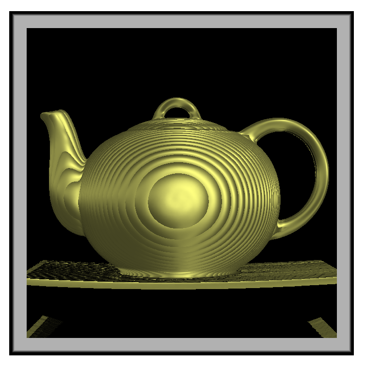
When writing your first volume renderer, you’ll undoubtedly come across the scourge of “wood grain” artifacts; your data will look like it’s made up of a stack of slices (which it is!). Obviously, reducing the raycast step size can help with this, but doing so can be detrimental to performance.
There are a couple popular tricks that can help: (1) re-checking the “solidity” of the voxel by jumping around at half-step intervals, and (2) jittering the ray’s starting position along the view direction. I added both of these tricks into our fragment shader; they’re highlighted in gray here:
// ...same as before...

uniform sampler2D Noise;

void main()
{
    // ...same as before...

    rayStart += stepVector * texture(Noise, gl_FragCoord.xy / 256).r;

    vec3 pos = rayStart;
    vec4 dst = vec4(0);
    while (dst.a < 1 && rayLength > 0) {

        float V = lookup(pos);
        if (V > Threshold) {

            vec3 s = -stepVector * 0.5;
            pos += s; V = lookup(pos);
            if (V > Threshold) s *= 0.5; else s *= -0.5;
            pos += s; V = lookup(pos);

            if (V > Threshold) {
                // ...same as before...
            }
        }

        pos += stepVector;
        rayLength -= StepLength;
    }

    FragColor = dst;
}
3D Gaussian Splat
Now that we’ve covered the basics of volume rendering, let’s come back to the main subject of this article, which deals with the generation of volumetric data using Gaussian splats.
One approach would be evaluating the 3D Gaussian function on the CPU during application initialization, and creating a 3D texture from that. However, I find it to be faster to simply compute the Gaussian in real-time, directly in the fragment shader.
Recall that we’re going to use instancing to render all the slices of the splat with only 1 draw call. One awkward aspect of GLSL is that the gl_InstanceID input variable is only accessible from the vertex shader, while the gl_Layer output variable is only accessible from the geometry shader. It’s not difficult to deal with this though! Without further ado, here’s the trinity of shaders for 3D Gaussian splatting:
-- Vertex Shader

in vec4 Position;
out vec2 vPosition;
out int vInstance;
uniform vec4 Center;

void main()
{
    gl_Position = Position + Center;
    vPosition = Position.xy;
    vInstance = gl_InstanceID;
}

-- Geometry Shader

layout(triangles) in;
layout(triangle_strip, max_vertices = 3) out;

in int vInstance[3];
in vec2 vPosition[3];
out vec3 gPosition;

uniform float InverseSize;

void main()
{
    gPosition.z = 1.0 - 2.0 * vInstance[0] * InverseSize;
    gl_Layer = vInstance[0];

    gPosition.xy = vPosition[0];
    gl_Position = gl_in[0].gl_Position;
    EmitVertex();

    gPosition.xy = vPosition[1];
    gl_Position = gl_in[1].gl_Position;
    EmitVertex();

    gPosition.xy = vPosition[2];
    gl_Position = gl_in[2].gl_Position;
    EmitVertex();

    EndPrimitive();
}

-- Fragment Shader

in vec3 gPosition;
out vec3 FragColor;

uniform vec3  Color;
uniform float InverseVariance;
uniform float NormalizationConstant;

void main()
{
    float r2 = dot(gPosition, gPosition);
    FragColor = Color * NormalizationConstant * exp(r2 * InverseVariance);
}
Setting up a 3D texture as a render target might be new to you; here’s one way you could set up the FBO: (note that I’m calling glFramebufferTexture rather than glFramebufferTexture{2,3}D)
struct Volume {
    GLuint FboHandle;
    GLuint TextureHandle;
};

Volume CreateVolume(GLsizei width, GLsizei height, GLsizei depth)
{
    Volume volume;
    glGenFramebuffers(1, &volume.FboHandle);
    glBindFramebuffer(GL_FRAMEBUFFER, volume.FboHandle);

    GLuint textureHandle;
    glGenTextures(1, &textureHandle);
    glBindTexture(GL_TEXTURE_3D, textureHandle);
    glTexParameteri(GL_TEXTURE_3D, GL_TEXTURE_WRAP_S, GL_CLAMP_TO_EDGE);
    glTexParameteri(GL_TEXTURE_3D, GL_TEXTURE_WRAP_T, GL_CLAMP_TO_EDGE);
    glTexParameteri(GL_TEXTURE_3D, GL_TEXTURE_WRAP_R, GL_CLAMP_TO_EDGE);
    glTexParameteri(GL_TEXTURE_3D, GL_TEXTURE_MIN_FILTER, GL_LINEAR);
    glTexParameteri(GL_TEXTURE_3D, GL_TEXTURE_MAG_FILTER, GL_LINEAR);
    glTexImage3D(GL_TEXTURE_3D, 0, GL_RGB16F, width, height, depth, 0,
                 GL_RGB, GL_HALF_FLOAT, 0);
    volume.TextureHandle = textureHandle;

    GLint miplevel = 0;
    GLuint colorbuffer;
    glGenRenderbuffers(1, &colorbuffer);
    glBindRenderbuffer(GL_RENDERBUFFER, colorbuffer);
    glFramebufferTexture(GL_FRAMEBUFFER, GL_COLOR_ATTACHMENT0, textureHandle, miplevel);

    return volume;
}
Note that we created a half-float RGB texture for volume rendering — this might seem like egregious usage of memory, but keep in mind that our end goal is to create a field of velocity vectors.
Flowline Extrusion
Now that we have the splat shaders ready, we can write the C++ code that extrudes a vector of positions into a velocity field. It works by looping over the positions in the path, computing the velocity at that point, and splatting the velocity. The call to glDrawArraysInstanced is simply rendering a quad with the instance count set to the depth of the splat.
typedef std::vector<VectorMath::Point3> PointList;

glEnable(GL_BLEND);
glBlendFunc(GL_ONE, GL_ONE);

PointList::const_iterator i = positions.begin();
for (; i != positions.end(); ++i) {

    PointList::const_iterator next = i;
    if (++next == positions.end())
        next = positions.begin();
    VectorMath::Vector3 velocity = (*next - *i);

    GLint center = glGetUniformLocation(program, "Center");
    glUniform4f(center, i->getX(), i->getY(), i->getZ(), 0);

    GLint color = glGetUniformLocation(program, "Color");
    glUniform3fv(color, 1, (float*) &velocity);

    glDrawArraysInstanced(GL_TRIANGLE_STRIP, 0, 4, Size);
}
Blending is essential for this to work correctly. If you want to create a true distance field, you’d want to use GL_MAX blending rather than the default blending equation (which is GL_FUNC_ADD), and you’d want your fragment shader to use evaluate a linear falloff rather than the Gaussian function.
Velocity Visualization
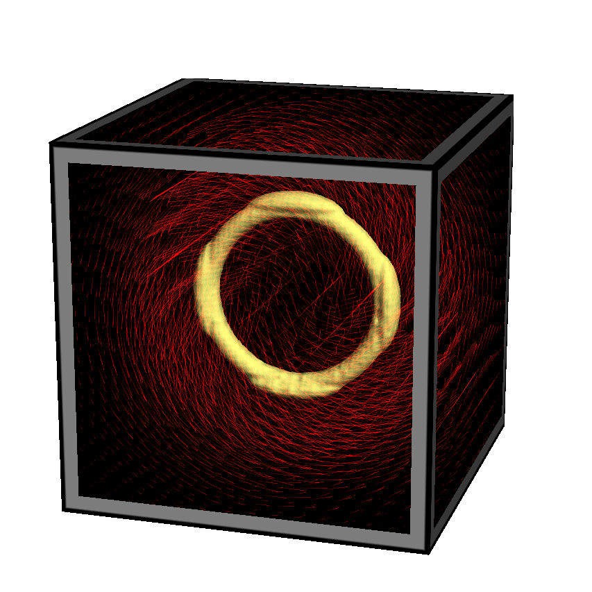
One popular way to visualize a grid of velocities is via short lines with alpha gradients, as in the image to the right (click to enlarge). This technique is easy to implement with modern OpenGL. Simply populate a VBO with a single point per grid cell, then use the geometry shader to extrude each point into a short line segment whose length and direction reflects the velocity vector in that cell. It’s rather beautiful actually! Here’s the shader triplet:
-- Vertex Shader

in vec4 Position;
out vec4 vPosition;
uniform mat4 ModelviewProjection;

void main()
{
    gl_Position = ModelviewProjection * Position;
    vPosition = Position;
}

-- Geometry Shader

layout(points) in;
layout(line_strip, max_vertices = 2) out;
out float gAlpha;
uniform mat4 ModelviewProjection;
in vec4 vPosition[1];
uniform sampler3D Volume;

void main()
{
    vec3 coord = 0.5 * (vPosition[0].xyz + 1.0);
    vec4 V = vec4(texture(Volume, coord).xyz, 0.0);

    gAlpha = 0;
    gl_Position = gl_in[0].gl_Position;
    EmitVertex();

    gAlpha = 1;
    gl_Position = ModelviewProjection * (vPosition[0] + V);
    EmitVertex();

    EndPrimitive();
}

-- Fragment Shader

out vec4 FragColor;
in float gAlpha;
uniform float Brightness = 0.5;

void main()
{
    FragColor = Brightness * vec4(gAlpha, 0, 0, 1);
}
Downloads
The demo code uses a subset of the Pez ecosystem, which is included in the zip below. It uses CMake for the build system.
I consider this code to be on the public domain. Enjoy!
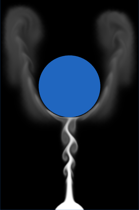
Simple Fluid Simulation
I finally wrote my first fluid simulation: two-dimensional smoke advected with GLSL fragment shaders. It was great fun, but let me warn you: it’s all too easy to drain away vast swaths of your life while tuning the millions of various parameters, just to get the right effect. It’s also rather addictive.
For my implementation, I used the classic Mark Harris article from GPU Gems 1 as my trusty guide. His article is available online here. Ah, 2004 seems like it was only yesterday…
Mark’s article is about a method called Eulerian Grid. In general, fluid simulation algorithms can be divided into three categories:
- Eulerian
-
Divides a cuboid of space into cells. Each cell contains a velocity vector and other information, such as density and temperature.
- Lagrangian
-
Particle-based physics, not as effective as Eulerian Grid for modeling “swirlies”. However, particles are much better for expansive regions, since they aren’t restricted to a grid.
- Hybrid
-
For large worlds that have specific regions where swirlies are desirable, use Lagrangian everywhere, but also place Eulerian grids in the regions of interest. When particles enter those regions, they become influenced by the grid’s velocity vectors. Jonathan Cohen has done some interesting work in this area.
Regardless of the method, the Navier-Stokes equation is at the root of it all. I won’t cover it here since you can read about it from a trillion different sources, all of which are far more authoritative than this blog. I’m focusing on implementation.
After reading Mark’s article, I found it useful to create a quick graphviz diagram for all the image processing:
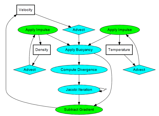
It’s not as complicated as it looks. The processing stages are all drawing full-screen quads with surprisingly simple fragment shaders. There are a total of three floating-point surfaces being processed: Velocity (a 2-component texture), Density (a 1-component texture), and Temperature (another 1-component texture).
In practice, you’ll need six surfaces instead of three; this allows ping-ponging between render targets and source textures. In some cases you can use blending instead; those stages are shown in green.
The processing stages are:
- Advect
-
Copies a quantity from a neighboring cell into the current cell; projects the current velocity backwards to find the incoming value. This is used for any type of quantity, including density, temperature, and velocity itself.
- Apply Impulse
-
This stage accounts for external forces, such as user interaction or the immortal candle in my simulation.
- Apply Buoyancy
-
For smoke effects, temperature can influence velocity by making it rise. In my implementation, I also apply the weight of the smoke in this stage; high densities in cool regions will sink.
- Compute Divergence
-
This stage computes values for a temporary surface (think of it as “scratch space”) that’s required for computing the pressure component of the Navier-Stokes equation.
- Jacobi Iteration
-
This is the real meat of the algorithm; it requires many iterations to converge to a good pressure value. The number of iterations is one of the many tweakables that I referred to at the beginning of this post, and I found that ~40 iterations was a reasonable number.
- Subtract Gradient
-
In this stage, the gradient of the pressure gets subtracted from velocity.
The above list is by no means set in stone — there are many ways to create a fluid simulation. For example, the Buoyancy stage is not necessary for liquids. Also, many simulations have a Vorticity Confinement stage to better preserve curliness, which I decided to omit. I also left out a Viscous Diffusion stage, since it’s not very useful for smoke.
Dealing with obstacles is tricky. One way of enforcing boundary conditions is adding a new operation after every processing stage. The new operation executes a special draw call that only touches the pixels that need to be tweaked to keep Navier-Stokes happy.
Alternatively, you can perform boundary enforcement within your existing fragment shaders. This adds costly texture lookups, but makes it easier to handle dynamic boundaries, and it simplifies your top-level image processing logic. Here’s the new diagram that takes obstacles into account: (alas, we can no longer use blending for SubtractGradient)
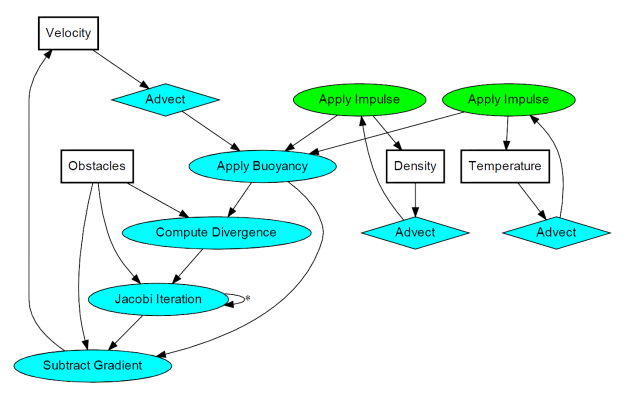
Note that I added a new surface called Obstacles. It has three components: the red component is essentially a boolean for solid versus empty, and the green/blue channels represent the obstacle’s velocity.
For my C/C++ code, I defined tiny POD structures for the various surfaces, and simple functions for each processing stage. This makes the top-level rendering routine easy to follow:
struct Surface {
    GLuint FboHandle;
    GLuint TextureHandle;
    int NumComponents;
};

struct Slab {
    Surface Ping;
    Surface Pong;
};

Slab Velocity, Density, Pressure, Temperature;
Surface Divergence, Obstacles;

// [snip]

glViewport(0, 0, GridWidth, GridHeight);

Advect(Velocity.Ping, Velocity.Ping, Obstacles, Velocity.Pong, VelocityDissipation);
SwapSurfaces(&Velocity);

Advect(Velocity.Ping, Temperature.Ping, Obstacles, Temperature.Pong, TemperatureDissipation);
SwapSurfaces(&Temperature);

Advect(Velocity.Ping, Density.Ping, Obstacles, Density.Pong, DensityDissipation);
SwapSurfaces(&Density);

ApplyBuoyancy(Velocity.Ping, Temperature.Ping, Density.Ping, Velocity.Pong);
SwapSurfaces(&Velocity);

ApplyImpulse(Temperature.Ping, ImpulsePosition, ImpulseTemperature);
ApplyImpulse(Density.Ping, ImpulsePosition, ImpulseDensity);

ComputeDivergence(Velocity.Ping, Obstacles, Divergence);
ClearSurface(Pressure.Ping, 0);

for (int i = 0; i < NumJacobiIterations; ++i) {
    Jacobi(Pressure.Ping, Divergence, Obstacles, Pressure.Pong);
    SwapSurfaces(&Pressure);
}

SubtractGradient(Velocity.Ping, Pressure.Ping, Obstacles, Velocity.Pong);
SwapSurfaces(&Velocity);
For my full source code, you can download the zip at the end of this article, but I’ll go ahead and give you a peek at the fragment shader for one of the processing stages. Like I said earlier, these shaders are mathematically simple on their own. I bet most of the performance cost is in the texture lookups, not the math. Here’s the shader for the Advect stage:
out vec4 FragColor;

uniform sampler2D VelocityTexture;
uniform sampler2D SourceTexture;
uniform sampler2D Obstacles;

uniform vec2 InverseSize;
uniform float TimeStep;
uniform float Dissipation;

void main()
{
    vec2 fragCoord = gl_FragCoord.xy;
    float solid = texture(Obstacles, InverseSize * fragCoord).x;
    if (solid > 0) {
        FragColor = vec4(0);
        return;
    }

    vec2 u = texture(VelocityTexture, InverseSize * fragCoord).xy;
    vec2 coord = InverseSize * (fragCoord - TimeStep * u);
    FragColor = Dissipation * texture(SourceTexture, coord);
}
Downloads
 The demo code uses a subset of the Pez ecosystem, which is included in the zip below. It can be built with Visual Studio 2010 or gcc. For the latter, I provided a WAF script instead of a makefile.
I consider this code to be on the public domain. Enjoy!
Path Instancing
Instancing and skinning are like peas and carrots. But remember, skinning isn’t the only way to deform a mesh on the GPU. In some situations, (for example, rendering aquatic life), a bone system can be overkill. If you’ve got a predefined curve in 3-space, it’s easy to write a vertex shader that performs path-based deformation.
Path-based deformation is obviously more limited than true skinning, but gives you the same performance benefits (namely, your mesh lives in an immutable VBO in graphics memory), and it is simpler to set up; no fuss over bone matrices.
Ideally your curve has two sets of data points: a set of node centers and a set of orientation vectors. Your first thought might be to store them in an array of shader uniforms, but don’t forget that modern vertex shaders can make texture lookups. It just so happens that these two sets of data can be nicely represented by a pair of rows in an RGB floating-point texture, like so:

Here’s the beauty part: by creating your texture with a GL_LINEAR filter, you’ll be able to leverage dedicated interpolation hardware to obtain points (and orientation vectors) that live between the node centers. (Component-wise lerping of orientation vectors isn’t quite mathematically kosher, but who’s watching?)
But wait, there’s more! Even the wrap modes of your texture will come in handy. If your 3-space curve is a closed loop, you can use GL_REPEAT for your S coordinate, and voilà — your shader need not worry its little head about cylindrical wrapping!
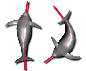
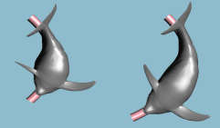
One gotcha with paths is that you’ll want to enforce an even spacing between nodes; this helps keep your shader simple. If your shader assumes a uniform distribution of path nodes, your models can become alarmingly foreshortened. For example, here’s a dolphin that’s tied to an elliptical path, before and after node re-distribution:
Now, without further ado, here’s my vertex shader. Note the complete lack of trig functions; I can’t tell you how many times I’ve seen graphics code that makes costly sine and cosine calls when simple linear algebra will suffice. I’m using old-school GLSL (e.g., attribute instead of in) to make my demo more amenable to Mac OS X.
attribute vec3 Position;
uniform mat4 ModelviewProjection;
uniform sampler2D Sampler;

uniform float TextureHeight;
uniform float InverseWidth;
uniform float InverseHeight;

uniform float PathOffset;
uniform float PathScale;

uniform int InstanceOffset;

void main()
{
    float id = gl_InstanceID + InstanceOffset;
    float xstep = InverseWidth;
    float ystep = InverseHeight;
    float xoffset = 0.5 * xstep;
    float yoffset = 0.5 * ystep;

    // Look up the current and previous centerline positions:
    vec2 texCoord;
    texCoord.x = PathScale * Position.x + PathOffset + xoffset;
    texCoord.y = 2.0 * id / TextureHeight + yoffset;
    vec3 currentCenter = texture2D(Sampler, texCoord).rgb;
    vec3 previousCenter = texture2D(Sampler, texCoord - vec2(xstep, 0)).rgb;

    // Next, compute the path direction vector.  Note that this
    // can be optimized by removing the normalize, if you know the node spacing.
    vec3 pathDirection = normalize(currentCenter - previousCenter);

    // Look up the current orientation vector:
    texCoord.x = PathOffset + xoffset;
    texCoord.y = texCoord.y + ystep;
    vec3 pathNormal = texture2D(Sampler, texCoord).rgb;

    // Form the change-of-basis matrix:
    vec3 a = pathDirection;
    vec3 b = pathNormal;
    vec3 c = cross(a, b);
    mat3 basis = mat3(a, b, c);

    // Transform the positions:
    vec3 spoke = vec3(0, Position.yz);
    vec3 position = currentCenter + basis * spoke;
    gl_Position = ModelviewProjection * vec4(position, 1);
}
The shader assumes that the undeformed mesh sits at the origin, with its spine aligned to the X axis. The way it works is this: first, compute the three basis vectors for a new coordinate system defined by the path segment. Next, place the basis vectors into a 3×3 matrix. Finally, apply the 3×3 matrix to the spoke vector, which goes from the mesh’s spine out to the current mesh vertex. Easy!
By the way, don’t feel ashamed if you’ve never made an instanced draw call with OpenGL before. It’s a relatively new feature that was added to the core in OpenGL 3.1. Before that, it was known as GL_ARB_draw_instanced. At the time of this writing, it’s still not supported on Mac OS X. Here’s how you do it with an indexed array:
glDrawElementsInstanced(GL_TRIANGLES, faceCount*3, GL_UNSIGNED_INT, 0, instanceCount);
When making this call, OpenGL automatically sets up the gl_InstanceID variable, which can be accessed from your vertex shader. Simple!
Downloads
The demo code uses a subset of the Pez ecosystem, which is included in the zip below. It uses a cool python-based build system called WAF. I tested it in a MinGW environment on a Windows 7 machine.
I consider this code to be on the public domain. Here’s a little video of the demo:
Silhouette Extraction
Some of my previous entries used the geometry shader (GS) to highlight certain triangle edges by passing new information to the fragment shader. The GS can also be used generate long, thin quads along those edges; this lets you apply texturing for sketchy effects. In the case of silhouette lines, you can create an anti-aliased border along the boundary of the model, without the cost of true multisampling.
In this article, I’ll show how to generate silhouettes using GLSL geometry shaders. At the end of the article, I provide the complete demo code for drawing the dragon depicted here. I tested the demo with Ubuntu (gcc), and Windows (Visual Studio 2010).
Old School Silhouettes
Just for fun, I want to point out a classic two-pass method for generating silhouettes, used in the days before shaders. I wouldn’t recommend it nowadays; it does not highlight creases and “core” OpenGL no longer supports smooth/wide lines anyway. This technique can be found in Under the Shade of the Rendering Tree by John Lander:
- Draw front faces:
- glPolygonMode(GL_FRONT, GL_FILL)
- glDepthFunc(GL_LESS)
- Draw back faces:
- glPolygonMode(GL_BACK, GL_LINE)
- glDepthFunc(GL_LEQUAL)
Ah, brings back memories…
Computing Adjacency
To detect silhouettes and creases, the GS examines the facet normals of adjacent triangles. So, we’ll need to send down the verts using GL_TRIANGLES_ADJACENCY:
glDrawElements(GL_TRIANGLES_ADJACENCY, // primitive type
               triangleCount*6,        // index count
               GL_UNSIGNED_SHORT,      // index type
               0);                     // start index
Six verts per triangle seems like an egregious redundancy of data, but keep in mind that it enlarges your index VBO, not your attributes VBO.
Typical mesh files don’t include adjacency information, but it’s easy enough to compute in your application. A wonderfully simple data structure for algorithms like this is the Half-Edge Table.
For low-level mesh algorithms, I enjoy using C99 rather than C++. I find that avoiding STL makes life a bit easier when debugging, and it encourages me to use memory efficiently. Here’s a half-edge structure in C:
typedef struct HalfEdgeRec
{
    unsigned short Vert;      // Vertex index at the end of this half-edge
    struct HalfEdgeRec* Twin; // Oppositely oriented adjacent half-edge
    struct HalfEdgeRec* Next; // Next half-edge around the face
} HalfEdge;
If you’ve got a half-edge structure for your mesh, it’s a simple linear-time algorithm to expand an index buffer to include adjacency information. Check out the downloads section to see how I did it.
By the way, you do need an associative array to build a half-edge table when loading model data from a traditional mesh file. In C++, this is all too easy because of helpful libraries like std::hash_map and Google’s Sparse Hash. For C99, I find that Judy arrays provide a compelling way of creating associative arrays.
Basic Fins
Now that we’ve got preliminaries out of the way, let’s start on the silhouette extrusion algorithm. We’ll start simple and make enhancements in the coming sections. We’ll use this torus as the demo model. The image on the left shows the starting point; the image on the right is our goal.

Silhouette lines occur on the boundary between front-facing triangles and back-facing triangles. Let’s define a function that takes three triangle corners (in screen space), returning true for front-facing triangles. To pull this off, we can take the cross product of two sides. If the Z component of the result is positive, then it’s front-facing. Since we can ignore the X and Y components of the result, this reduces to:
bool IsFront(vec2 A, vec2 B, vec2 C)
{
    return 0 < (A.x * B.y - B.x * A.y) + (B.x * C.y - C.x * B.y) + (C.x * A.y - A.x * C.y);
}
Incidentally, the length of the cross-product is equal to twice the area of the triangle. But I digress…
The next function emits a long, thin quadrilateral between two points. To do this, we’ll add an extrusion vector to the two endpoints. In the following snippet, N is the extrusion vector, computed by taking the perpendicular of the normalized vector between the two points, then scaling it by half the desired line width:
uniform float HalfWidth;

void EmitEdge(vec2 P0, vec2 P1)
{
    vec2 V = normalize(P1 - P0);
    vec2 N = vec2(-V.y, V.x) * HalfWidth;

    gl_Position = vec4(P0 - N, 0, 1); EmitVertex();
    gl_Position = vec4(P0 + N, 0, 1); EmitVertex();
    gl_Position = vec4(P1 - N, 0, 1); EmitVertex();
    gl_Position = vec4(P1 + N, 0, 1); EmitVertex();
    EndPrimitive();
}
Next let’s write main() for the geometry shader. It checks if the current triangle is frontfacing, then emits a quad for each backfacing neighbor:
layout(triangles_adjacency) in;
layout(triangle_strip, max_vertices = 12) out;

void main()
{
    vec2 v0 = gl_in[0].gl_Position.xy;
    vec2 v1 = gl_in[1].gl_Position.xy;
    vec2 v2 = gl_in[2].gl_Position.xy;
    vec2 v3 = gl_in[3].gl_Position.xy;
    vec2 v4 = gl_in[4].gl_Position.xy;
    vec2 v5 = gl_in[5].gl_Position.xy;

    if (IsFront(v0, v2, v4)) {
        if (!IsFront(v0, v1, v2)) EmitEdge(v0, v2);
        if (!IsFront(v2, v3, v4)) EmitEdge(v2, v4);
        if (!IsFront(v0, v4, v5)) EmitEdge(v4, v0);
    }
}
Here’s the result:
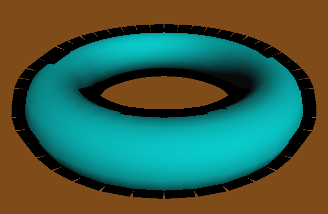
Not too pretty. There are three problems with this silhouette:
- The outer edge of the fin needs some antialiasing.
- We’re only seeing the upper half of the fin.
- There’s a gap between neighboring fins.
We’ll address each of these issues in the coming sections.
Antialiased Fins
First let’s add some antialiasing to those fins. To pull this off, we’ll attach a distance-from-center value to each corner of the quad. In the fragment shader, we can use these values to see how far the current pixel is from the edge. If it’s less than a couple pixels away, it fades the alpha value. The EmitEdge function now becomes:
out float gDist;
uniform float HalfWidth;

void EmitEdge(vec2 P0, vec2 P1)
{
    vec2 V = normalize(P1 - P0);
    vec2 N = vec2(-V.y, V.x) * HalfWidth;

    gDist = +HalfWidth;
    gl_Position = vec4(P0 - N, 0, 1); EmitVertex();
    gDist = -HalfWidth;
    gl_Position = vec4(P0 + N, 0, 1); EmitVertex();
    gDist = +HalfWidth;
    gl_Position = vec4(P1 - N, 0, 1); EmitVertex();
    gDist = -HalfWidth;
    gl_Position = vec4(P1 + N, 0, 1); EmitVertex();
    EndPrimitive();
}
Next is the fragment shader, which uses the tipLength variable to represent the length of the desired alpha gradient. We leverage GLSL’s built-in fwidth function to prevent it from looking fuzzy when zoomed in:
in float gDist;
out vec4 fColor;
uniform float HalfWidth;
const vec3 LineColor = vec3(0, 0, 0);

void main()
{
    float alpha = 1.0;
    float d = abs(gDist);
    float tipLength = 2.0 * fwidth(d);
    if (d > HalfWidth - tipLength)
        alpha = 1.0 - (d - HalfWidth + tipLength) / tipLength;

    fColor = vec4(LineColor, alpha);
}
Here’s the result:

The Spine Test
We extruded in both directions, so why are we seeing only half of the fin? The issue lies with depth testing. We could simply disable all depth testing during the silhouette pass, but then we’d see creases from the opposite side of the model. The correct trick is to perform depth testing along the centerline of the quad, rather than at the current fragment. This method is called spine testing, and it was introduced by a recent paper from Forrester Cole and Adam Finkelstein.
In order to perform custom depth testing, we’ll need to do an early Z pass. An early Z pass is often useful for other reasons, especially for scenes with high depth complexity. In our demo program, we generate a G-Buffer containing normals and depths:
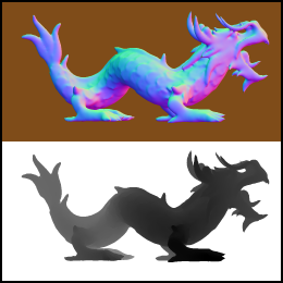
The normals are used for per-pixel lighting while the depths are used for spine testing. The fragment shader for G-Buffer generation is exceedingly simple; it simply transforms the normals into the [0,1] range and writes them out:
in vec3 vNormal;
out vec3 fColor;

void main()
{
    fColor = (vNormal + 1.0) * 0.5;
}
When rendering silhouette lines, the fragment shader will need texture coordinates for the spine. The geometry shader comes to the rescue again. It simply transforms the device coordinates of the quad’s endpoints into texture coordinates, then writes them out to a new output variable:
out float gDist;
out vec2 gSpine;
uniform float HalfWidth;

void EmitEdge(vec2 P0, vec2 P1)
{
    vec2 V = normalize(P1 - P0);
    vec2 N = vec2(-V.y, V.x) * HalfWidth;

    gSpine = (P0 + 1.0) * 0.5;
    gDist = +HalfWidth;
    gl_Position = vec4(P0 - N, 0, 1); EmitVertex();
    gDist = -HalfWidth;
    gl_Position = vec4(P0 + N, 0, 1); EmitVertex();
    gSpine = (P1 + 1.0) * 0.5;
    gDist = +HalfWidth;
    gl_Position = vec4(P1 - N, 0, 1); EmitVertex();
    gDist = -HalfWidth;
    gl_Position = vec4(P1 + N, 0, 1); EmitVertex();
    EndPrimitive();
}
Next we enhance the fragment shader to issue a discard for fragments that fail the custom depth test:
in float gDist;
in vec2 gSpine;
out vec4 fColor;
uniform float HalfWidth;
uniform sampler2D DepthSampler;
uniform vec2 Size;

void main()
{
    vec2 texCoord = gSpine;
    float depth = texture2D(DepthSampler, texCoord).r;
    if (depth < gl_FragCoord.z)
        discard;

    float alpha = 1.0;
    float d = abs(gDist);
    float tipLength = 2.0 * fwidth(d);
    if (d > HalfWidth - tipLength)
        alpha = 1.0 - (d - HalfWidth + tipLength) / tipLength;

    fColor = vec4(0, 0, 0, alpha);
}
Here’s the result. Note that the fin now extends below the contour, allowing you to see the AA on both ends.
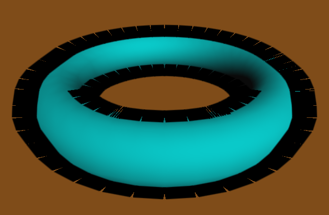
Mind the Gap!
Next let’s fill in those gaps, creating the illusion of a single, seamless line. Some researchers create new triangles on either end of the fin, using vertex normals to determine the shape of those triangles. In practice I found this tricky to work with, especially since vertex normals are usually intended for 3D lighting, not screen-space effects. I found it easier to simply extend the lengths of the quads that I’m already generating. Sure, this causes too much overlap in some places, but it doesn’t seem to hurt the final image quality much. The percentage by which to extend the fin length is controlled via the OverhangLength shader uniform in the following snippet:
out float gDist;
out vec2 gSpine;
uniform float HalfWidth;
uniform float OverhangLength;

void EmitEdge(vec2 P0, vec2 P1)
{
    vec2 E = OverhangLength * (P1 - P0);
    vec2 V = normalize(E);
    vec2 N = vec2(-V.y, V.x) * HalfWidth;

    gSpine = (P0 + 1.0) * 0.5;
    gDist = +HalfWidth;
    gl_Position = vec4(P0 - N - E, 0, 1); EmitVertex();
    gDist = -HalfWidth;
    gl_Position = vec4(P0 + N - E, 0, 1); EmitVertex();
    gSpine = (P1 + 1.0) * 0.5;
    gDist = +HalfWidth;
    gl_Position = vec4(P1 - N + E, 0, 1); EmitVertex();
    gDist = -HalfWidth;
    gl_Position = vec4(P1 + N + E, 0, 1); EmitVertex();
    EndPrimitive();
}
Here’s the final result:
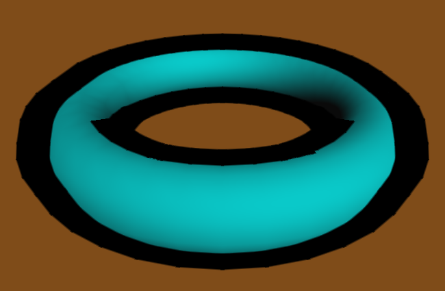
Further Reading
These are some of the resources that gave me ideas for this blog post:
- There’s a nice article at Gamasutra about silhouette rendering with DirectX 10, written by an old colleague of mine, Josh Doss.
- Achieving AA by drawing lines on top of the model is called edge overdraw, which was written about in this 2001 paper by Hughes Hoppe and others.
- My silhouette lines are centered at the boundary, rather than extending only in the outwards direction. To achieve this, I use the “spine test”, which was introduced in a nice paper entitled Two Fast Methods for High-Quality Line Visibility, by Forrester Cole and Adam Finkelstein.
- To learn how to generate texture coordinates for fins (e.g., sketchy lines), and a different way of dealing with the gap between fins, check out a paper entitled Single Pass GPU Stylized Edges, by Hermosilla and Vázquez.
Downloads
The demo code uses a subset of the Pez ecosystem, which is included in the zip below.
I consider this code to be on the public domain.
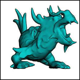
Thick Glass with Floating-Point Textures
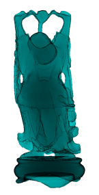
This post covers a simple way to measure thickness and apply a Fresnel term using a floating-point render target. Sample OpenGL code is provided that runs on Snow Leopard and Windows.
There’s an excellent article in GPU Pro entitled Multi-Fragment Effects on the GPU Using Bucket Sort. This technique for order-independent transparency is useful for a variety of reasons, but I noticed that one of the applications they show off can be achieved in an easier way. You can measure thickness by simply making two depth-only passes into a floating-point texture; this is a technique that NVIDIA leveraged for some of their demos back in 2005. Here’s a nice presentation that shows how:
GPU Programming Exposed: The Naked Truth Behind NVIDIA’s Demos
In olden times, you would’ve used the ARB_depth_texture extension for making depth-only passes like this, but nowadays I don’t see any reason for using a special extension. Simply bind a floating-point (or half-float) FBO and use a fragment shader that outputs gl_FragCoord.z.
You might be wondering why we need a floating-point texture for this, rather than a plain ol’ 8888 texture. Non-float textures can only represent intensities in the range [0, 1]. We need unclamped colors. Sure, we could normalize depth in the fragment shader, but that wouldn’t be enough for scenes with multiple layers of depth complexity. Consider viewing a donut edge-on; the backface pass would be accumulating twice. If we normalize to [0,1], the total accumulated depth could still be as high as 2.0.
So why not use 8888 and simply normalize depth to some small number, say 0.1? That would allow for 10 layers of depth complexity, no? Sure, but you’d run into precision artifacts real fast. (Trust me, I’ve tried it.) For a high-quality effect, it’s imperative to use a floating-point render target.
Thickness
Update: Andreas Vasilakis astutely pointed out that this can be done in only one pass if you simply leverage the gl_FrontFacing built-in varying in your fragment shader and negate depth if you’re on a backface. Sweet! I’ve implemented this idea in WebGL here.
The principle is simple: turn on additive blending, then render front faces. Next, negate Z and render back faces. The resulting image represents thickness:
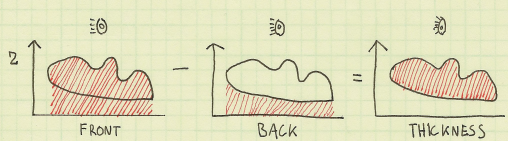
Here’s the C side code for how you can do this with OpenGL:
glEnable(GL_CULL_FACE);
glEnable(GL_BLEND);
glBlendFunc(GL_ONE, GL_ONE);
GLint depthScale = glGetUniformLocation(DepthProgram, "DepthScale");

// Draw front faces in the first pass:
glUniform1f(depthScale, 1.0f);
glCullFace(GL_BACK);
glDrawElements(GL_TRIANGLES, Buddha.FaceCount * 3, GL_UNSIGNED_SHORT, 0);

// Draw back faces in the first pass:
glUniform1f(depthScale, -1.0f);
glCullFace(GL_FRONT);
glDrawElements(GL_TRIANGLES, Buddha.FaceCount * 3, GL_UNSIGNED_SHORT, 0);
And here are the shaders. I’m using old-school GLSL syntax to be compatible with Mac OS X.
-- Vertex

attribute vec4 Position;
uniform mat4 Projection;
uniform mat4 Modelview;

void main()
{
    gl_Position = Projection * Modelview * Position;
}

-- Fragment

uniform float DepthScale;

void main()
{
    float depth = DepthScale * gl_FragCoord.z;
    gl_FragColor = vec4(depth, 0, 0, 0);
}
Simulating Light Absorption
Thickness alone isn’t enough for a nice glass effect though. It helps to apply Beer’s law in a final image processing pass:
I = exp(-sigma * thickness)
Sigma is the “absorption coefficient”. You’ll need to play around to find a nice value for your situation.
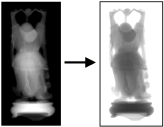
The following snippet shows off the image-processing shader. Note the sneaky usage of gl_FragCoord for obtaining texture coordinates; this lets us avoid the work of sending down texture coordinates just for a full-screen quad.
-- Vertex.Quad

attribute vec4 Position;

void main()
{
    gl_Position = Position;
}

-- Fragment.Absorption

uniform sampler2D Sampler;
uniform vec2 Size;
uniform vec3 Color;

void main()
{
    vec2 texCoord = gl_FragCoord.xy / Size;
    float thickness = abs(texture2D(Sampler, texCoord).r);
    if (thickness <= 0.0)
    {
        discard;
    }
    float sigma = 30.0;
    float intensity = exp(-sigma * thickness);
    gl_FragColor = vec4(intensity * Color, 1);
}
Fresnel
The Fresnel effect is a classic shader computation for making your glass even more realistic. We store thickness in the red channel and the Fresnel term in the green channel. We then subtract the Fresnel term during the image processing pass. You can visualize the subtraction like this:
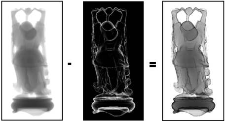
The vertex shader for drawing Buddha now sends out normals and eye-space positions:
-- Vertex

attribute vec4 Position;
attribute vec3 Normal;

varying vec3 vNormal;
varying vec3 vPosition;

uniform mat4 Projection;
uniform mat4 Modelview;
uniform mat3 NormalMatrix;

void main()
{
    vPosition = (Modelview * Position).xyz;
    vNormal = NormalMatrix * Normal;
    gl_Position = Projection * Modelview * Position;
}
We can apply the Fresnel calculation in the fragment shader and write it out to the green channel like so:
-- Fragment.Depth

uniform float DepthScale;
varying vec3 vNormal;
varying vec3 vPosition;

void main()
{
    vec3 N = normalize(vNormal);
    vec3 P = vPosition;
    vec3 I = normalize(P);
    float cosTheta = abs(dot(I, N));
    float fresnel = pow(1.0 - cosTheta, 4.0);

    float depth = DepthScale * gl_FragCoord.z;

    gl_FragColor = vec4(depth, fresnel, 0, 0);
}
Here’s the new image processing pass that accounts for the Fresnel term:
-- Vertex.Quad

attribute vec4 Position;

void main()
{
    gl_Position = Position;
}

-- Fragment.Absorption

uniform sampler2D Sampler;
uniform vec2 Size;
uniform vec3 Color;

void main()
{
    vec2 texCoord = gl_FragCoord.xy / Size;
    float thickness = abs(texture2D(Sampler, texCoord).r);
    if (thickness <= 0.0)
    {
        discard;
    }
    float sigma = 30.0;
    float fresnel = 1.0 - texture2D(Sampler, texCoord).g;
    float intensity = fresnel * exp(-sigma * thickness);
    gl_FragColor = vec4(intensity * Color, 1);
}
Downloads
Everything is provided to build and run on Snow Leopard with Xcode, or Windows with Visual Studio 2010.
I consider this code to be on the public domain.
Quad Tessellation with OpenGL 4.0
This is the second of a two-part article on tessellation shaders with OpenGL 4.0+. This entry walks through simple bezier patch subdivision; the previous entry gave an overview of tessellation and triangle subdivision. This article is going to be short and sweet.
You might also want to review my article on patch evaluation in Python, and Ken Perlin’s course notes on patches.
Quad Subdivision
Whenever implementing a tessellation scheme, I find it best to initially get things going without any smoothing. In other words, simply divide up the patch without introducing any curvature. Here’s how our demo renders Catmull’s Gumbo model using the subdivided-but-not-smoothed approach:
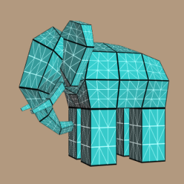
To generate a simple subdivision image like this, the tessellation evaluation shader needs to consider only the 4 corners of the patch. Since we’re using 16 control points per patch, the corners are at positions 0, 3, 12, and 15. All we have to do is lerp between those four verts, and here’s the tessellation evaluation shader for doing so:
-- TessEval

layout(quads) in;
in vec3 tcPosition[];
out vec3 tePosition;
uniform mat4 Projection;
uniform mat4 Modelview;

void main()
{
    float u = gl_TessCoord.x, v = gl_TessCoord.y;
    vec3 a = mix(tcPosition[0], tcPosition[3], u);
    vec3 b = mix(tcPosition[12], tcPosition[15], u);
    tePosition = mix(a, b, v);
    gl_Position = Projection * Modelview * vec4(tePosition, 1);
}
If you’re wondering about the strange prefixes on variables like tcPosition, flip back to the previous entry.
Bezier Smoothing
Of course, we can make Gumbo more rounded by performing proper smoothing, in which case we can obtain an image like this:
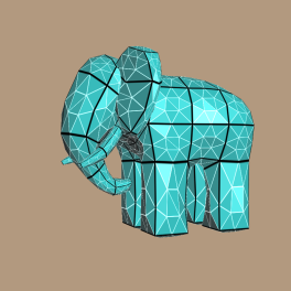
Here’s the final version of the tessellation evaluation shader:
-- TessEval

layout(quads) in;
in vec3 tcPosition[];
out vec3 tePosition;
out vec4 tePatchDistance;
uniform mat4 Projection;
uniform mat4 Modelview;
uniform mat4 B;
uniform mat4 BT;

void main()
{
    float u = gl_TessCoord.x, v = gl_TessCoord.y;

    mat4 Px = mat4(
        tcPosition[0].x, tcPosition[1].x, tcPosition[2].x, tcPosition[3].x,
        tcPosition[4].x, tcPosition[5].x, tcPosition[6].x, tcPosition[7].x,
        tcPosition[8].x, tcPosition[9].x, tcPosition[10].x, tcPosition[11].x,
        tcPosition[12].x, tcPosition[13].x, tcPosition[14].x, tcPosition[15].x );

    mat4 Py = mat4(
        tcPosition[0].y, tcPosition[1].y, tcPosition[2].y, tcPosition[3].y,
        tcPosition[4].y, tcPosition[5].y, tcPosition[6].y, tcPosition[7].y,
        tcPosition[8].y, tcPosition[9].y, tcPosition[10].y, tcPosition[11].y,
        tcPosition[12].y, tcPosition[13].y, tcPosition[14].y, tcPosition[15].y );

    mat4 Pz = mat4(
        tcPosition[0].z, tcPosition[1].z, tcPosition[2].z, tcPosition[3].z,
        tcPosition[4].z, tcPosition[5].z, tcPosition[6].z, tcPosition[7].z,
        tcPosition[8].z, tcPosition[9].z, tcPosition[10].z, tcPosition[11].z,
        tcPosition[12].z, tcPosition[13].z, tcPosition[14].z, tcPosition[15].z );

    mat4 cx = B * Px * BT;
    mat4 cy = B * Py * BT;
    mat4 cz = B * Pz * BT;

    vec4 U = vec4(u*u*u, u*u, u, 1);
    vec4 V = vec4(v*v*v, v*v, v, 1);

    float x = dot(cx * V, U);
    float y = dot(cy * V, U);
    float z = dot(cz * V, U);
    tePosition =  vec3(x, y, z);

    tePatchDistance = vec4(u, v, 1-u, 1-v);
    gl_Position = Projection * Modelview * vec4(x, y, z, 1);
}
The above shader pretty much does exactly what the Python script in my other blog entry does. Note that I also write out a vec4 of edge distances to the tePatchDistance output variable; these are used for the wireframe technique, which I’ll cover shortly.
Of course, this isn’t very efficient. Some of the calculations are being performed at every vertex, but really they only need to performed once per patch. Namely, computation of the coefficient matrices (cx, cy, and cz) should be hoisted up into the tessellation control shader. Then, tcPosition can become a representation of those matrices, rather than being coordinates for the raw control points. Alas, I ran into driver / compiler issues when I made this optimization. OpenGL 4.0 is still a young technology, and the drivers need some time to mature. I’ll dig deeper when I have time, and file bug reports against the hardware vendor that I’m using.
Black and White Lines
You may have noticed that I improved on the wireframe technique presented in my previous blog entry; I now render the triangle edges in white, and the patch edges in black. The geometry shader is exactly the same as what I presented earlier:
-- Geometry

uniform mat4 Modelview;
uniform mat3 NormalMatrix;
layout(triangles) in;
layout(triangle_strip, max_vertices = 3) out;
in vec3 tePosition[3];
in vec4 tePatchDistance[3];
out vec3 gFacetNormal;
out vec4 gPatchDistance;
out vec3 gTriDistance;

void main()
{
    vec3 A = tePosition[2] - tePosition[0];
    vec3 B = tePosition[1] - tePosition[0];
    gFacetNormal = NormalMatrix * normalize(cross(A, B));

    gPatchDistance = tePatchDistance[0];
    gTriDistance = vec3(1, 0, 0);
    gl_Position = gl_in[0].gl_Position; EmitVertex();

    gPatchDistance = tePatchDistance[1];
    gTriDistance = vec3(0, 1, 0);
    gl_Position = gl_in[1].gl_Position; EmitVertex();

    gPatchDistance = tePatchDistance[2];
    gTriDistance = vec3(0, 0, 1);
    gl_Position = gl_in[2].gl_Position; EmitVertex();

    EndPrimitive();
}
The fragment shader is almost the same, except that I’m taking the min of four distances for the patch edges. I’m also drawing triangle edges in white, and I snuck in a specular component to the lighting computation:
-- Fragment

out vec4 FragColor;
in vec3 gFacetNormal;
in vec3 gTriDistance;
in vec4 gPatchDistance;
uniform vec3 LightPosition;
uniform vec3 DiffuseMaterial;
uniform vec3 AmbientMaterial;
uniform vec3 SpecularMaterial;
uniform float Shininess;
const vec3 InnerLineColor = vec3(1, 1, 1);
const bool DrawLines = false;

float amplify(float d, float scale, float offset)
{
    d = scale * d + offset;
    d = clamp(d, 0, 1);
    d = 1 - exp2(-2*d*d);
    return d;
}

void main()
{
    vec3 N = normalize(gFacetNormal);
    vec3 L = LightPosition;
    vec3 E = vec3(0, 0, 1);
    vec3 H = normalize(L + E);

    float df = abs(dot(N, L));
    float sf = abs(dot(N, H));
    sf = pow(sf, Shininess);
    vec3 color = AmbientMaterial + df * DiffuseMaterial + sf * SpecularMaterial;

    if (DrawLines) {
        float d1 = min(min(gTriDistance.x, gTriDistance.y), gTriDistance.z);
        float d2 = min(min(min(gPatchDistance.x, gPatchDistance.y), gPatchDistance.z), gPatchDistance.w);
        d1 = 1 - amplify(d1, 50, -0.5);
        d2 = amplify(d2, 50, -0.5);
        color = d2 * color + d1 * d2 * InnerLineColor;
    }

    FragColor = vec4(color, 1.0);
}
That’s about it! Here’s Gumbo with per-facet normals, but with DrawLines turned off:
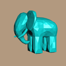
Downloads
The demo code uses a subset of the Pez ecosystem, which is included in the zip below. (The Pez ecosystem is a handful of tiny libraries whose source is included directly in the project.)
I consider this code to be on the public domain. To run it, you’ll need CMake, a very up-to-date graphics driver, and a very modern graphics card.
Triangle Tessellation with OpenGL 4.0
This is the first of a two-part article on tessellation shaders with OpenGL 4.0+. This entry gives an overview of tessellation and walks through an example of simple triangle subdivision; in the next entry, we’ll focus on quad subdivision.
Reviewing Geometry Shaders
When Geometry Shaders (GS) first came out, we were all excited because we could finally write a shader that could “see” all the verts in a triangle at once. And finally, the GPU could produce more primitives than it consumed.
The GS unit turned out to be convenient for certain effects, but overall it was somewhat disappointing. It was not designed for large-scale amplification of vertex data. The GS processing for a single primitive was initially limited to a single processing unit. Most GS programs had a serial loop that simply pushed out the verts of the new primitive(s), one vertex after another. They didn’t do a great job of leveraging the massive parallelism in GPUs. Nowadays you can do a bit better by specifying an invocations count at the top of your GS, like so:
layout(triangles, invocations = 3) in;
This tells the GPU that your GS should run three times on a single primitive. You can figure out which vert you’re on by looking at the built-in gl_InvocationID variable.
The New OpenGL 4.0+ Pipeline
Although adding multiple GS invocations was helpful, performing highly-efficient subdivision demanded brand new stages in the pipeline. Now is the time for the obligatory diagram: (I used a red pen for the stages that are new to OpenGL 4.0)
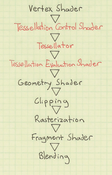
So, we now have two additional programmable stages at our disposal: Tessellation Control and Tessellation Evaluation. They both execute on a per-vertex basis, so their programs typically don’t have serial loops like the old-fashioned geometry programs did. However, much like geometry shaders, they can “see” all the verts in a single primitive.
To work with tessellation shaders, OpenGL now has a new primitive type: GL_PATCHES. Unlike GL_TRIANGLES (where every 3 verts spawns a triangle) or GL_TRIANGLE_STRIP (where every 1 vert spawns a new triangle), the number of verts in a patch is configurable:
glPatchParameteri(GL_PATCH_VERTICES, 16);       // tell OpenGL that every patch has 16 verts
glDrawArrays(GL_PATCHES, firstVert, vertCount); // draw a bunch of patches
The Tessellation Control (TC) shader is kinda like a Vertex Shader (VS) with super-vision. Much like a VS program, each TC program transforms only one vertex, and the number of execution instances is the same as the number of verts in your OpenGL draw call. The Tessellation Evaluation (TE) shader, however, usually processes more verts than you sent down in your draw call. That’s because the “Tessellator” (the stage between the two new shaders) generates brand new verts by interpolating between the existing verts.
As the name implies, the TC shader has some control over how the Tessellator generates new verts. This is done through the gl_TessLevelInner and gl_TessLevelOuter output variables. More on these later.
Another way of controlling how the Tessellator generates verts is through the layout qualifier on the TE shader’s inputs. You’ll often see a TE shader with something like this at the top:
layout(triangles, equal_spacing, cw) in;
This specifies three things: a primitive mode, a vertex spacing, and an ordering. The latter two are optional and they have reasonable defaults — I won’t go into detail about them here. As for the primitive mode, there are three choices: triangles, quads, and isolines. As mentioned earlier, in this article I’ll focus on triangles; for more on quads, see my next article.
Inner and Outer Tess Levels
Simply put, the inner tessellation level controls the number of “nested” primitives, and the outer tessellation level controls the number of times to subdivide each edge. The gl_TessLevelInner and gl_TessLevelOuter variable are both arrays-of-float, but with triangle subdivision, there’s only one element in the inner array. The outer array has three elements, one for each side of the triangle. In both arrays, a value of 1 indicates no subdivision whatsoever. For the inner tess level, a value of 2 means that there’s only one nested triangle, but it’s degenerate; it’s just a single point. It’s not till tess level 3 that you see a miniatured of the original triangle inside the original triangle.
Since the tess levels are controlled at the shader level (as opposed to the OpenGL API level), you can do awesome things with dynamic level-of-detail. However, for demonstration purposes, we’ll limit ourselves to the simple case here. We’ll set the inner tess level to a hardcoded value, regardless of distance-from-camera. For the outer tess level, we’ll set all three edges to the same value. Here’s a little diagram that shows how triangle-to-triangle subdivision can be configured with our demo program, which sends an icosahedron to OpenGL:
| Inner = 1 | Inner = 2 | Inner = 3 | Inner = 4 | |
| Outer = 1 | 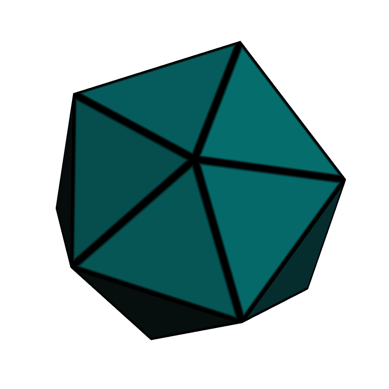 |
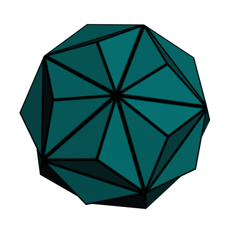 |
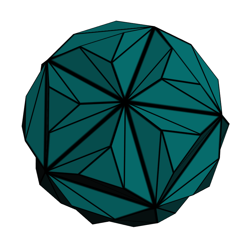 |
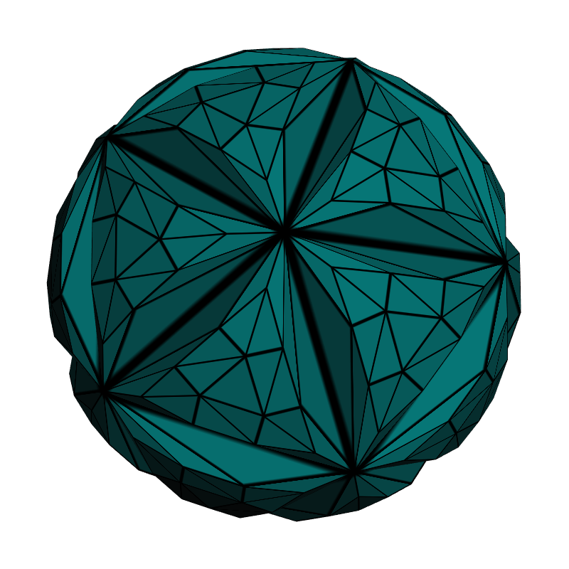 |
| Outer = 2 | 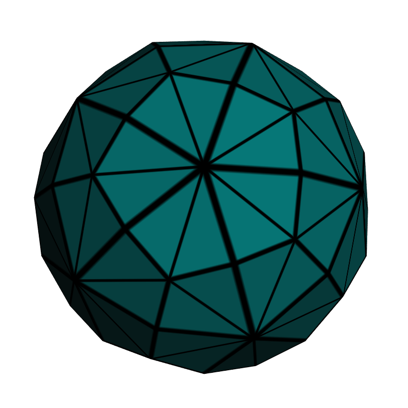 |
 |
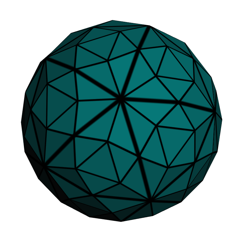 |
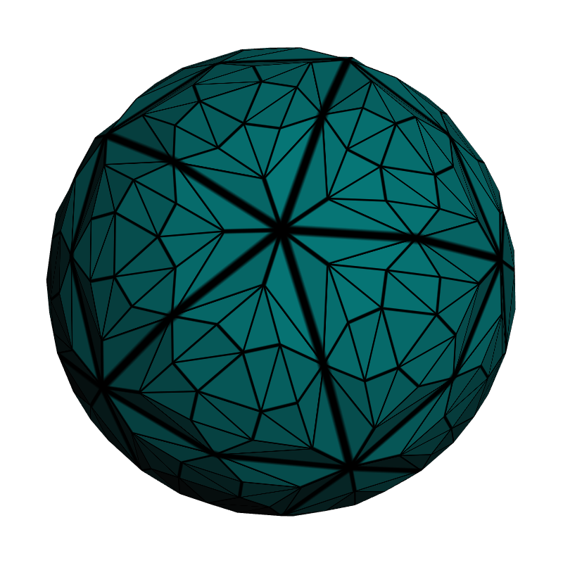 |
| Outer = 3 |  |
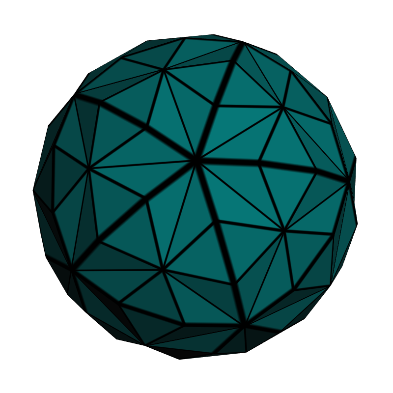 |
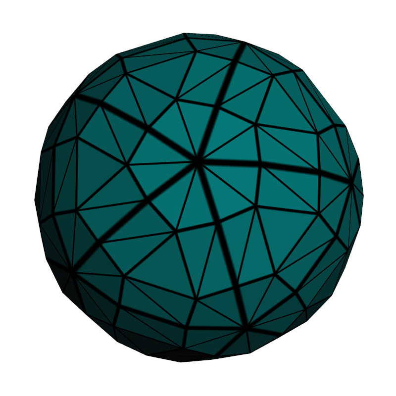 |
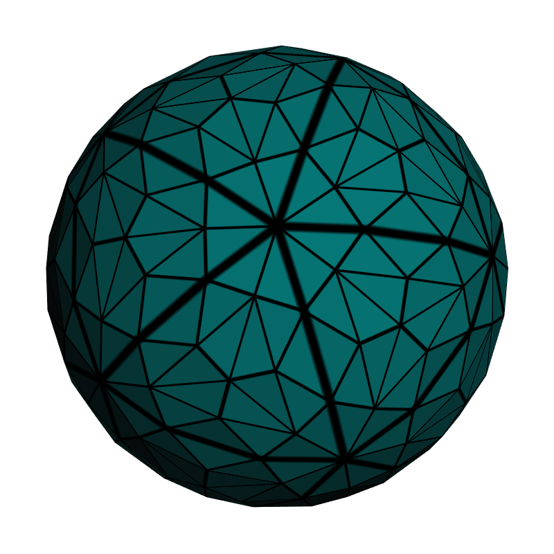 |
| Outer = 4 | 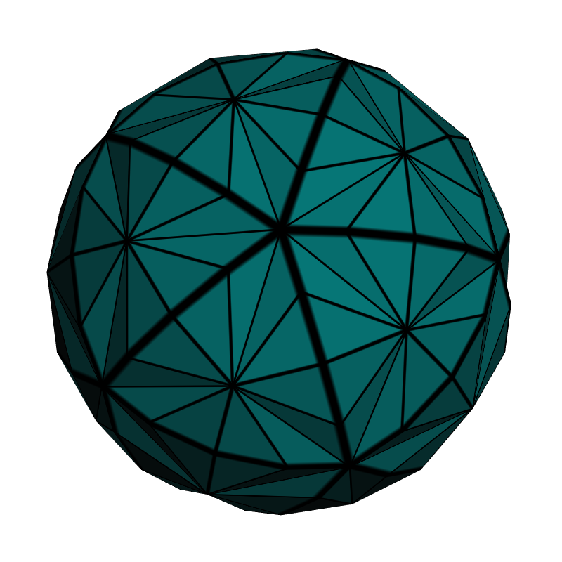 |
 |
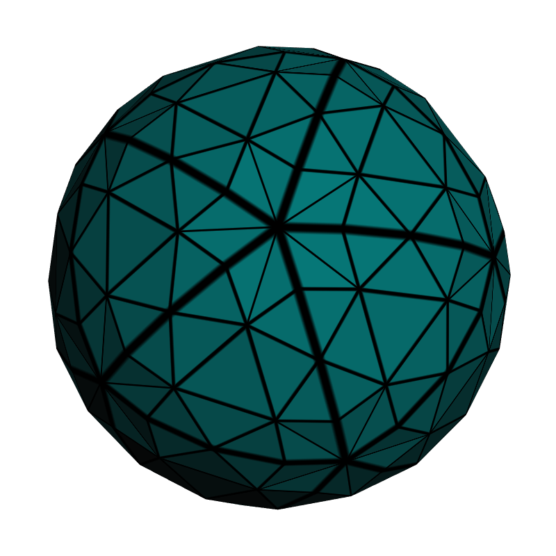 |
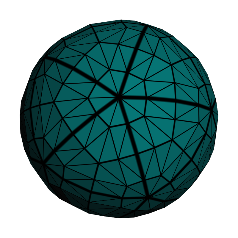 |
Show Me The Code
Building the VAO for the icosahedron isn’t the subject of this article, but for completeness here’s the C code for doing so:
static void CreateIcosahedron()
{
    const int Faces[] = {
        2, 1, 0,
        3, 2, 0,
        4, 3, 0,
        5, 4, 0,
        1, 5, 0,
        11, 6,  7,
        11, 7,  8,
        11, 8,  9,
        11, 9,  10,
        11, 10, 6,
        1, 2, 6,
        2, 3, 7,
        3, 4, 8,
        4, 5, 9,
        5, 1, 10,
        2,  7, 6,
        3,  8, 7,
        4,  9, 8,
        5, 10, 9,
        1, 6, 10 };

    const float Verts[] = {
         0.000f,  0.000f,  1.000f,
         0.894f,  0.000f,  0.447f,
         0.276f,  0.851f,  0.447f,
        -0.724f,  0.526f,  0.447f,
        -0.724f, -0.526f,  0.447f,
         0.276f, -0.851f,  0.447f,
         0.724f,  0.526f, -0.447f,
        -0.276f,  0.851f, -0.447f,
        -0.894f,  0.000f, -0.447f,
        -0.276f, -0.851f, -0.447f,
         0.724f, -0.526f, -0.447f,
         0.000f,  0.000f, -1.000f };

    IndexCount = sizeof(Faces) / sizeof(Faces[0]);

    // Create the VAO:
    GLuint vao;
    glGenVertexArrays(1, &vao);
    glBindVertexArray(vao);

    // Create the VBO for positions:
    GLuint positions;
    GLsizei stride = 3 * sizeof(float);
    glGenBuffers(1, &positions);
    glBindBuffer(GL_ARRAY_BUFFER, positions);
    glBufferData(GL_ARRAY_BUFFER, sizeof(Verts), Verts, GL_STATIC_DRAW);
    glEnableVertexAttribArray(PositionSlot);
    glVertexAttribPointer(PositionSlot, 3, GL_FLOAT, GL_FALSE, stride, 0);

    // Create the VBO for indices:
    GLuint indices;
    glGenBuffers(1, &indices);
    glBindBuffer(GL_ELEMENT_ARRAY_BUFFER, indices);
    glBufferData(GL_ELEMENT_ARRAY_BUFFER, sizeof(Faces), Faces, GL_STATIC_DRAW);
}
Our vertex shader is even more boring:
-- Vertex

in vec4 Position;
out vec3 vPosition;

void main()
{
    vPosition = Position.xyz;
}
We use a special naming convention for in/out variables. If we need to trickle Foo through the entire pipeline, here’s how we avoid naming collisions:
- Foo is the original vertex attribute (sent from the CPU)
- vFoo is the output of the VS and the input to the TC shader
- tcFoo is the output of the TC shader and the input to the TE shader
- teFoo is the output of the TE shader and the input to the GS
- gFoo is the output of the GS and the input to the FS
Now, without further ado, we’re ready to show off our tessellation control shader:
-- TessControl

layout(vertices = 3) out;
in vec3 vPosition[];
out vec3 tcPosition[];
uniform float TessLevelInner;
uniform float TessLevelOuter;

#define ID gl_InvocationID

void main()
{
    tcPosition[ID] = vPosition[ID];
    if (ID == 0) {
        gl_TessLevelInner[0] = TessLevelInner;
        gl_TessLevelOuter[0] = TessLevelOuter;
        gl_TessLevelOuter[1] = TessLevelOuter;
        gl_TessLevelOuter[2] = TessLevelOuter;
    }
}
That’s almost as boring as our vertex shader! Note that per-patch outputs (such as gl_TessLevelInner) only need to be written once. We enclose them in an if so that we only bother writing to them from a single execution thread. Incidentally, you can create custom per-patch variables if you’d like; simply use the patch out qualifier when declaring them.
Here’s the tessellation control shader that we use for our icosahedron demo:
-- TessEval

layout(triangles, equal_spacing, cw) in;
in vec3 tcPosition[];
out vec3 tePosition;
out vec3 tePatchDistance;
uniform mat4 Projection;
uniform mat4 Modelview;

void main()
{
    vec3 p0 = gl_TessCoord.x * tcPosition[0];
    vec3 p1 = gl_TessCoord.y * tcPosition[1];
    vec3 p2 = gl_TessCoord.z * tcPosition[2];
    tePatchDistance = gl_TessCoord;
    tePosition = normalize(p0 + p1 + p2);
    gl_Position = Projection * Modelview * vec4(tePosition, 1);
}
The built-in gl_TessCoord variable lets us know where we are within the patch. In this case, the primitive mode is triangles, so gl_TessCoord is a barycentric coordinate. If we were performing quad subdivision, then it would be a UV coordinate and we’d ignore the Z component.
Our demo subdivides the icosahedron in such a way that it approaches a perfect unit sphere, so we use normalize to push the new verts onto the sphere’s surface.
The tePatchDistance output variable will be used by the fragment shader to visualize the edges of the patch; this brings us to the next section.
Geometry Shaders Are Still Fun!
Geometry shaders are now considered the runt of the litter, but sometimes they’re useful for certain techniques, like computing facet normals on the fly, or creating a nice single-pass wireframe. In this demo, we’ll do both. We’re intentionally using non-smooth normals (in other words, the lighting is the same across the triangle) because it helps visualize the tessellation.
For a brief overview on rendering nice wireframes with geometry shaders, check out this SIGGRAPH sketch. To summarize, the GS needs to send out a vec3 “edge distance” at each corner; these automatically get interpolated by the rasterizer, which gives the fragment shader a way to determine how far the current pixel is from the nearest edge.
We’ll extend the wireframe technique here because we wish the pixel shader to highlight two types of edges differently. The edge of the final triangle is drawn with a thin line, and the edge of the original patch is drawn with a thick line.
-- Geometry

uniform mat4 Modelview;
uniform mat3 NormalMatrix;
layout(triangles) in;
layout(triangle_strip, max_vertices = 3) out;
in vec3 tePosition[3];
in vec3 tePatchDistance[3];
out vec3 gFacetNormal;
out vec3 gPatchDistance;
out vec3 gTriDistance;

void main()
{
    vec3 A = tePosition[2] - tePosition[0];
    vec3 B = tePosition[1] - tePosition[0];
    gFacetNormal = NormalMatrix * normalize(cross(A, B));

    gPatchDistance = tePatchDistance[0];
    gTriDistance = vec3(1, 0, 0);
    gl_Position = gl_in[0].gl_Position; EmitVertex();

    gPatchDistance = tePatchDistance[1];
    gTriDistance = vec3(0, 1, 0);
    gl_Position = gl_in[1].gl_Position; EmitVertex();

    gPatchDistance = tePatchDistance[2];
    gTriDistance = vec3(0, 0, 1);
    gl_Position = gl_in[2].gl_Position; EmitVertex();

    EndPrimitive();
}
As you can see, we used the classic one-at-a-time method in our GS, rather than specifying an invocations count other than 1. This is fine for demo purposes.
Our fragment shader does some per-pixel lighting (which is admittedly silly; the normal is the same across the triangle, so we should’ve performed lighting much earlier) and takes the minimum of all incoming distances to see if the current pixel lies near an edge.
out vec4 FragColor;
in vec3 gFacetNormal;
in vec3 gTriDistance;
in vec3 gPatchDistance;
in float gPrimitive;
uniform vec3 LightPosition;
uniform vec3 DiffuseMaterial;
uniform vec3 AmbientMaterial;

float amplify(float d, float scale, float offset)
{
    d = scale * d + offset;
    d = clamp(d, 0, 1);
    d = 1 - exp2(-2*d*d);
    return d;
}

void main()
{
    vec3 N = normalize(gFacetNormal);
    vec3 L = LightPosition;
    float df = abs(dot(N, L));
    vec3 color = AmbientMaterial + df * DiffuseMaterial;

    float d1 = min(min(gTriDistance.x, gTriDistance.y), gTriDistance.z);
    float d2 = min(min(gPatchDistance.x, gPatchDistance.y), gPatchDistance.z);
    color = amplify(d1, 40, -0.5) * amplify(d2, 60, -0.5) * color;

    FragColor = vec4(color, 1.0);
}
That completes the shader code for the demo, and we managed to specify code for all of the five shader stages in the modern GPU pipeline. Here’s the final output using a tessellation level of 4 for both inner and outer:
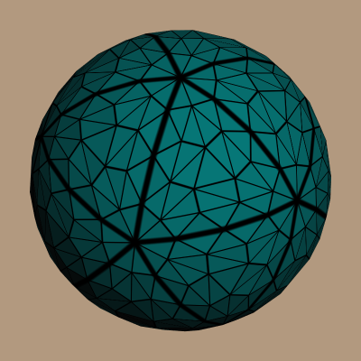
Downloads
The demo code uses a subset of the Pez ecosystem, which is included in the zip below. (The Pez ecosystem is a handful of tiny libraries whose source is included directly in the project).
I consider this code to be on the public domain. To run it, you’ll need CMake, a very up-to-date graphics driver, and a very modern graphics card. Good luck!
“iPhone 3D” In Stock At Amazon!
Amazon has replaced the Pre-order button for my book with Add to Cart. To celebrate, I created a word cloud of the entire book using wordle.net and a python script. Here’s the word cloud:
I love that “API” got nestled into “ES”. To create the word cloud, I first ran a little python script against the book’s DocBook source. The script simply extracts content from para elements. If I don’t do this, the word cloud contains all the sample code and represents words like const in huge, overwhelming text. (I tried it, trust me.) Anyway here’s the script:
from xml.dom.minidom import parse
import codecs

def getText(nodelist):
    rc = ""
    for node in nodelist:
        if node.nodeType == node.TEXT_NODE:
            rc = rc + node.data
    return rc

f = codecs.open( "wordle.txt", "w", "utf-8" )

for i in xrange(0, 10):
    filename = "ch%02d.xml" % i
    tree = parse(filename)
    paras = tree.getElementsByTagName("para")
    for para in paras:
        f.write(getText(para.childNodes))

print "wordle.txt has been dumped"
After running the script, I simply pasted the resulting text file into wordle.net.
PEZ: A Teeny Tiny GLUT Alternative
Pez enables cross-platform development of extremely simple OpenGL apps. It’s not really a library since it’s so small. Instead of linking it in, just plop one of these files into your project:
You’ll also need a single header file:
Like GLUT, Pez lets you quickly build simple OpenGL apps that will run on any platform. Unlike GLUT, it never makes any OpenGL calls on your behalf. This makes it easy to write demos that conform to the forward-compatible profile in OpenGL 3.0+.
Pez doesn’t require you to register callbacks like GLUT does. Instead, your program simply provides definitions for four functions:
// receive window size and return window title
const char* PezInitialize(int width, int height);

// draw scene (Pez swaps the backbuffer for you)
void PezRender();

// receive elapsed time (e.g., update physics)
void PezUpdate(unsigned int milliseconds);

// handle mouse action: PEZ_DOWN, PEZ_UP, or PEZ_MOVE
void PezHandleMouse(int x, int y, int action);
That’s it! Pez defines main() (or WinMain on Microsoft platforms) and runs a game loop for you. Additionally, Pez defines a handful of utility functions that serve as alternatives to printf, exceptions, and asserts:
void PezDebugString(const char* pStr, ...);
void PezDebugStringW(const wchar_t* pStr, ...);
void PezFatalError(const char* pStr, ...);
void PezFatalErrorW(const wchar_t* pStr, ...);
#define PezCheckCondition(A, B) if (!(A)) { PezFatalError(B); }
#define PezCheckConditionW(A, B) if (!(A)) { PezFatalErrorW(B); }

On Windows, strings get sent to the debugger, so use the VS debugger window or dbgview to see them.
Pez doesn’t handle keyboard stuff and resizable windows. If you want to do anything fancy, just edit the Pez source and treat it as a starting point. Pez is written in ANSI C and released under the MIT License.
The only outside library that Pez depends on is GLEW, which is also so tiny that you can plop it down directly into your project. Usage of glew is especially nice on Windows platforms, since it lets you avoid including the huge windows.h header, and it loads up function pointers on your behalf. Pez calls glewInit() for you.
GLEW is included in the downloadable Pez package at the end of the post, along with a few other super-light libraries such as GLSW and pnglite. Together, these libraries form the “Pez Ecosystem”, which I’ll discuss later. You don’t need to use the entire ecosystem to use Pez; GLEW is the only required library.
You can configure some aspects of Pez (most importantly, window size) by editing pez.h and modifying one of these constants:
#define PEZ_VIEWPORT_WIDTH 853
#define PEZ_VIEWPORT_HEIGHT 480
#define PEZ_ENABLE_MULTISAMPLING 1
#define PEZ_VERTICAL_SYNC 1
Simple Example
Here’s a little flashlight app that oscillates the background color and becomes bright yellow when pressing a mouse button. Note that it includes glew.h rather than gl.h.
#include <pez.h>
#include <glew.h>
#include <math.h>

static float elapsed = 0;
static int pressing = 0;
static float speed = 0.01f;

const char* PezInitialize(int width, int height)
{
    return "Pez Intro";
}

void PezRender()
{
    if (pressing) {
        glClearColor(1, 1, 0.75f, 1);
    } else {
        float blue = 0.5f * (1.0f + sinf(elapsed));
        glClearColor(0, 0.25f, blue, 1);
    }
    glClear(GL_COLOR_BUFFER_BIT);
}

void PezUpdate(unsigned int elapsedMilliseconds)
{
    elapsed += elapsedMilliseconds * speed;
}

void PezHandleMouse(int x, int y, int action)
{
    if (action == PEZ_DOWN)
        pressing = 1;
    else if (action == PEZ_UP)
        pressing = 0;
}
Hello Triangle
Next let’s try something a bit more complex:
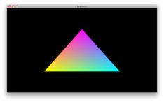
Here are the source files for this demo:
Since we’re using modern OpenGL, even a simple task like this requires the usage of shaders. First let’s write the effect file:
-- Vertex.GL3

in vec2 Position;
in vec3 InColor;
out vec3 OutColor;

void main()
{
    OutColor = InColor;
    gl_Position = vec4(Position, 0, 1);
}

-- Fragment.GL3

in vec3 OutColor;
out vec4 FragColor;

void main()
{
    FragColor = vec4(OutColor, 1);
}
The gray ‘--’ section dividers are not legal in the shading language, but they get parsed out by GLSW. Let’s move on to the C code:
#include <pez.h>
#include <glew.h>
#include <glsw.h>

static void BuildGeometry();
static void LoadEffect();

enum { PositionSlot, ColorSlot };

void PezHandleMouse(int x, int y, int action) { }

void PezUpdate(unsigned int elapsedMilliseconds) { }

void PezRender()
{
    glClear(GL_COLOR_BUFFER_BIT);
    glDrawArrays(GL_TRIANGLES, 0, 3);
}

const char* PezInitialize(int width, int height)
{
    BuildGeometry();
    LoadEffect();
    return "Pez Intro";
}
Note that I used a static qualifier on the forward declarations of BuildGeometry() and LoadEffect(); this emphasizes the fact that they’re private to this file.
Let’s go ahead and implement BuildGeometry(), which creates a VBO for the triangle and enables a couple vertex attributes (position and color):
static void BuildGeometry()
{
    float verts[] = {
        -0.5f, -0.5f,  1,1,0, // Yellow
        +0.0f, +0.5f,  1,0,1, // Magenta
        +0.5f, -0.5f,  0,1,1, // Cyan
    };

    GLuint vboHandle;
    GLsizeiptr vboSize = sizeof(verts);
    GLsizei stride = 5 * sizeof(float);
    GLenum usage = GL_STATIC_DRAW;
    GLvoid* colorOffset = (GLvoid*) (sizeof(float) * 2);

    glGenBuffers(1, &vboHandle);
    glBindBuffer(GL_ARRAY_BUFFER, vboHandle);
    glBufferData(GL_ARRAY_BUFFER, vboSize, verts, usage);
    glVertexAttribPointer(PositionSlot, 2, GL_FLOAT, GL_FALSE, stride, 0);
    glVertexAttribPointer(ColorSlot, 3, GL_FLOAT, GL_FALSE, stride, colorOffset);
    glEnableVertexAttribArray(PositionSlot);
    glEnableVertexAttribArray(ColorSlot);
}
Next we’ll write the code that fetches a pair of shaders from GLSW, compiles them, binds the color and position slots, and links them together to form a program object:
static void LoadEffect()
{
    const char* vsSource, * fsSource;
    GLuint vsHandle, fsHandle;
    GLint compileSuccess, linkSuccess;
    GLchar compilerSpew[256];
    GLuint programHandle;

    glswInit();
    glswSetPath("../demo/", ".glsl");
    glswAddDirectiveToken("GL3", "#version 130");

    vsSource = glswGetShader("Simple.Vertex." PEZ_GL_VERSION_TOKEN);
    fsSource = glswGetShader("Simple.Fragment." PEZ_GL_VERSION_TOKEN);
    PezCheckCondition(vsSource, "Can't find vertex shader.\n");
    PezCheckCondition(fsSource, "Can't find fragment shader.\n");

    vsHandle = glCreateShader(GL_VERTEX_SHADER);
    fsHandle = glCreateShader(GL_FRAGMENT_SHADER);

    glShaderSource(vsHandle, 1, &vsSource, 0);
    glCompileShader(vsHandle);
    glGetShaderiv(vsHandle, GL_COMPILE_STATUS, &compileSuccess);
    glGetShaderInfoLog(vsHandle, sizeof(compilerSpew), 0, compilerSpew);
    PezCheckCondition(compileSuccess, compilerSpew);

    glShaderSource(fsHandle, 1, &fsSource, 0);
    glCompileShader(fsHandle);
    glGetShaderiv(fsHandle, GL_COMPILE_STATUS, &compileSuccess);
    glGetShaderInfoLog(fsHandle, sizeof(compilerSpew), 0, compilerSpew);
    PezCheckCondition(compileSuccess, compilerSpew);

    programHandle = glCreateProgram();
    glAttachShader(programHandle, vsHandle);
    glAttachShader(programHandle, fsHandle);
    glBindAttribLocation(programHandle, PositionSlot, "Position");
    glBindAttribLocation(programHandle, ColorSlot, "Color");
    glLinkProgram(programHandle);
    glGetProgramiv(programHandle, GL_LINK_STATUS, &linkSuccess);
    glGetProgramInfoLog(programHandle, sizeof(compilerSpew), 0, compilerSpew);
    PezCheckCondition(linkSuccess, compilerSpew);

    glUseProgram(programHandle);
}
That’s it!
Ghandi Texture
Next we’ll write a tiny Pez program that loads a PNG texture and draws it to the screen:
Here are the source files for this demo:
Aside from Pez itself, so far we’ve pulled in two other libraries to facilitate our sample code: GLEW and GLSW. We’re slowly forming the “Pez Ecosystem” that I’ll cover later. We now need a library to help us load textures from an external file. I like pnglite since it’s yet another “one C file, one H file” solution. Here’s how to use pnglite to load in our Gandhi texture:
static void LoadTexture()
{
    png_t tex;
    unsigned char* data;
    GLuint textureHandle;

    png_init(0, 0);
    png_open_file_read(&tex, "../demo/Gandhi.png");
    data = (unsigned char*) malloc(tex.width * tex.height * tex.bpp);
    png_get_data(&tex, data);

    glGenTextures(1, &textureHandle);
    glBindTexture(GL_TEXTURE_2D, textureHandle);
    glTexImage2D(GL_TEXTURE_2D, 0, GL_RGB, tex.width, tex.height, 0,
                 GL_RGB, GL_UNSIGNED_BYTE, data);
    glTexParameteri(GL_TEXTURE_2D, GL_TEXTURE_MIN_FILTER, GL_LINEAR);
    glTexParameteri(GL_TEXTURE_2D, GL_TEXTURE_MAG_FILTER, GL_LINEAR);

    png_close_file(&tex);
    free(data);
}
The above code assumes that the PNG image is RGB only (does not contain alpha). I don’t advise hardcoding stuff like this in production code, but we’re just listing out some simple examples. Here’s the effect file:
-- Vertex.Textured.GL3

in vec2 Position;
in vec2 InCoord;
out vec2 OutCoord;

void main()
{
    OutCoord = InCoord;
    gl_Position = vec4(Position, 0, 1);
}

-- Fragment.Textured.GL3

in vec2 OutCoord;
out vec4 FragColor;
uniform sampler2D Sampler;

void main()
{
    FragColor = texture(Sampler, OutCoord);
}
The C source looks like this:
#include <pez.h>
#include <glew.h>
#include <glsw.h>
#include <pnglite.h>
#include <stdlib.h>

static void BuildGeometry();
static void LoadEffect();
static void LoadTexture();

enum { PositionSlot, TexCoordSlot };

void PezHandleMouse(int x, int y, int action) { }

void PezUpdate(unsigned int elapsedMilliseconds) { }

void PezRender()
{
    glClear(GL_COLOR_BUFFER_BIT);
    glDrawArrays(GL_TRIANGLES, 0, 6);
}

const char* PezInitialize(int width, int height)
{
    BuildGeometry();
    LoadEffect();
    LoadTexture();
    return "Pez Intro";
}

static void LoadTexture()
{
    // ...see previous listing for implementation...
}

static void BuildGeometry()
{
    #define X (0.5f * PEZ_VIEWPORT_HEIGHT / PEZ_VIEWPORT_WIDTH)
    #define Y (0.5f)
    float verts[] = {
        -X, -Y,  0,1,
        -X, +Y,  0,0,
        +X, +Y,  1,0,
        +X, +Y,  1,0,
        +X, -Y,  1,1,
        -X, -Y,  0,1,
    };
    #undef X
    #undef Y

    GLuint vboHandle;
    GLsizeiptr vboSize = sizeof(verts);
    GLsizei stride = 4 * sizeof(float);
    GLenum usage = GL_STATIC_DRAW;
    GLvoid* texCoordOffset = (GLvoid*) (sizeof(float) * 2);

    glGenBuffers(1, &vboHandle);
    glBindBuffer(GL_ARRAY_BUFFER, vboHandle);
    glBufferData(GL_ARRAY_BUFFER, vboSize, verts, usage);
    glVertexAttribPointer(PositionSlot, 2, GL_FLOAT, GL_FALSE, stride, 0);
    glVertexAttribPointer(TexCoordSlot, 2, GL_FLOAT, GL_FALSE, stride, texCoordOffset);
    glEnableVertexAttribArray(PositionSlot);
    glEnableVertexAttribArray(TexCoordSlot);
}

static void LoadEffect()
{
    const char* vsSource, * fsSource;
    GLuint vsHandle, fsHandle;
    GLint compileSuccess, linkSuccess;
    GLchar compilerSpew[256];
    GLuint programHandle;

    glswInit();
    glswSetPath("../demo/", ".glsl");
    glswAddDirectiveToken("GL3", "#version 130");

    vsSource = glswGetShader("Simple.Vertex.Textured." PEZ_GL_VERSION_TOKEN);
    fsSource = glswGetShader("Simple.Fragment.Textured." PEZ_GL_VERSION_TOKEN);
    PezCheckCondition(vsSource, "Can't find vertex shader.\n");
    PezCheckCondition(fsSource, "Can't find fragment shader.\n");

    vsHandle = glCreateShader(GL_VERTEX_SHADER);
    fsHandle = glCreateShader(GL_FRAGMENT_SHADER);

    glShaderSource(vsHandle, 1, &vsSource, 0);
    glCompileShader(vsHandle);
    glGetShaderiv(vsHandle, GL_COMPILE_STATUS, &compileSuccess);
    glGetShaderInfoLog(vsHandle, sizeof(compilerSpew), 0, compilerSpew);
    PezCheckCondition(compileSuccess, compilerSpew);

    glShaderSource(fsHandle, 1, &fsSource, 0);
    glCompileShader(fsHandle);
    glGetShaderiv(fsHandle, GL_COMPILE_STATUS, &compileSuccess);
    glGetShaderInfoLog(fsHandle, sizeof(compilerSpew), 0, compilerSpew);
    PezCheckCondition(compileSuccess, compilerSpew);

    programHandle = glCreateProgram();
    glAttachShader(programHandle, vsHandle);
    glAttachShader(programHandle, fsHandle);
    glBindAttribLocation(programHandle, PositionSlot, "Position");
    glBindAttribLocation(programHandle, TexCoordSlot, "InCoord");
    glLinkProgram(programHandle);
    glGetProgramiv(programHandle, GL_LINK_STATUS, &linkSuccess);
    glGetProgramInfoLog(programHandle, sizeof(compilerSpew), 0, compilerSpew);
    PezCheckCondition(linkSuccess, compilerSpew);

    glUseProgram(programHandle);
}
That’s it for the texture viewer!
Mesh Viewer
Next let’s light up some artistic 3D content and spin it around:
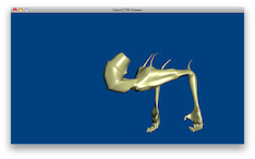
For this demo, we’ll switch from ANSI C to C++. Here are the source files:
For the per-pixel lighting effect, see my other blog post. For loading the “headless giant” mesh, we’ll use OpenCTM, which supports good compression and has a nice & simple API. Here’s how we’ll use it to load the model and create a VBO:
static void LoadMesh()
{
    RenderContext& rc = GlobalRenderContext;

    // Open the CTM file:
    CTMcontext ctmContext = ctmNewContext(CTM_IMPORT);
    ctmLoad(ctmContext, "../demo/HeadlessGiant.ctm");
    PezCheckCondition(ctmGetError(ctmContext) == CTM_NONE, "OpenCTM Issue");
    CTMuint vertexCount = ctmGetInteger(ctmContext, CTM_VERTEX_COUNT);
    rc.IndexCount = 3 * ctmGetInteger(ctmContext, CTM_TRIANGLE_COUNT);

    // Create the VBO for positions:
    const CTMfloat* positions = ctmGetFloatArray(ctmContext, CTM_VERTICES);
    if (positions) {
        GLuint handle;
        GLsizeiptr size = vertexCount * sizeof(float) * 3;
        glGenBuffers(1, &handle);
        glBindBuffer(GL_ARRAY_BUFFER, handle);
        glBufferData(GL_ARRAY_BUFFER, size, positions, GL_STATIC_DRAW);
        glEnableVertexAttribArray(SlotPosition);
        glVertexAttribPointer(SlotPosition, 3, GL_FLOAT, GL_FALSE, sizeof(float) * 3, 0);
    }

    // Create the VBO for normals:
    const CTMfloat* normals = ctmGetFloatArray(ctmContext, CTM_NORMALS);
    if (normals) {
        GLuint handle;
        GLsizeiptr size = vertexCount * sizeof(float) * 3;
        glGenBuffers(1, &handle);
        glBindBuffer(GL_ARRAY_BUFFER, handle);
        glBufferData(GL_ARRAY_BUFFER, size, normals, GL_STATIC_DRAW);
        glEnableVertexAttribArray(SlotNormal);
        glVertexAttribPointer(SlotNormal, 3, GL_FLOAT, GL_FALSE, sizeof(float) * 3, 0);
    }

    // Create the VBO for indices:
    const CTMuint* indices = ctmGetIntegerArray(ctmContext, CTM_INDICES);
    if (indices) {
        GLuint handle;
        GLsizeiptr size = rc.IndexCount * sizeof(CTMuint);
        glGenBuffers(1, &handle);
        glBindBuffer(GL_ELEMENT_ARRAY_BUFFER, handle);
        glBufferData(GL_ELEMENT_ARRAY_BUFFER, size, indices, GL_STATIC_DRAW);
    }

    ctmFreeContext(ctmContext);
}
The other lightweight library we’ll pull in for this example is the Sony Vector Library, which has nice APIs for C and C++, and supports the various matrix operations from old-school OpenGL that are no longer in the core specification. For example, here’s how you’d use their C++ API to compute a projection matrix from a viewing frustum:
Matrix4 projection = Matrix4::frustum(left, right, bottom, top, zNear, zFar);
The C++ source code for this demo is fairly straightforward. Here it is:
#include <pez.h>
#include <vectormath_aos.h>
#include <glsw.h>
#include <glew.h>
#include <openctm.h>

using namespace Vectormath::Aos;

enum { SlotPosition, SlotNormal };

struct ShaderUniforms {
    GLuint Projection;
    GLuint Modelview;
    GLuint NormalMatrix;
};

struct RenderContext {
    GLuint EffectHandle;
    ShaderUniforms EffectUniforms;
    Matrix4 Projection;
    Matrix4 Modelview;
    Matrix3 NormalMatrix;
    float PackedNormalMatrix[9];
    float Theta;
    CTMuint IndexCount;
};

static RenderContext GlobalRenderContext;
static GLuint BuildShader(const char* source, GLenum shaderType);
static GLuint BuildProgram(const char* vsKey, const char* fsKey);
static void LoadMesh();
static void LoadEffect();

void PezHandleMouse(int x, int y, int action) { }

const char* PezInitialize(int width, int height)
{
    LoadMesh();
    LoadEffect();
    glEnable(GL_DEPTH_TEST);
    return "OpenCTM Viewer";
}

void PezRender()
{
    RenderContext& rc = GlobalRenderContext;
    glClearColor(0, 0.25f, 0.5f, 1);
    glClear(GL_COLOR_BUFFER_BIT | GL_DEPTH_BUFFER_BIT);
    glUniformMatrix4fv(rc.EffectUniforms.Projection, 1, 0, &rc.Projection[0][0]);
    glUniformMatrix4fv(rc.EffectUniforms.Modelview, 1, 0, &rc.Modelview[0][0]);
    glUniformMatrix3fv(rc.EffectUniforms.NormalMatrix, 1, 0, &rc.PackedNormalMatrix[0]);
    glDrawElements(GL_TRIANGLES, rc.IndexCount, GL_UNSIGNED_INT, 0);
}

void PezUpdate(unsigned int elapsedMilliseconds)
{
    RenderContext& rc = GlobalRenderContext;

    rc.Theta += elapsedMilliseconds * 0.05f;

    Matrix4 rotation = Matrix4::rotationY(rc.Theta * Pi / 180.0f);
    Matrix4 translation = Matrix4::translation(Vector3(0, 0, -50));
    rc.Modelview = translation * rotation;
    rc.NormalMatrix = rc.Modelview.getUpper3x3();

    for (int i = 0; i < 9; ++i)
        rc.PackedNormalMatrix[i] = rc.NormalMatrix[i / 3][i % 3];

    const float x = 0.6f;
    const float y = x * PEZ_VIEWPORT_HEIGHT / PEZ_VIEWPORT_WIDTH;
    const float left = -x, right = x;
    const float bottom = -y, top = y;
    const float zNear = 4, zFar = 100;
    rc.Projection = Matrix4::frustum(left, right, bottom, top, zNear, zFar);
}

static void LoadMesh()
{
    // ...see previous listing for implementation...
}

static GLuint BuildShader(const char* source, GLenum shaderType)
{
    // ...similar to previous listings...
}

static GLuint BuildProgram(const char* vsKey, const char* fsKey)
{
    // ...similar to previous listings...
}

static void LoadEffect()
{
    RenderContext& rc = GlobalRenderContext;

    glswInit();
    glswSetPath("../demo/", ".glsl");
    glswAddDirectiveToken("GL3", "#version 130");

    const char* vsKey = "PixelLighting.Vertex." PEZ_GL_VERSION_TOKEN;
    const char* fsKey = "PixelLighting.Fragment." PEZ_GL_VERSION_TOKEN;

    rc.EffectHandle = BuildProgram(vsKey, fsKey);
    rc.EffectUniforms.Projection = glGetUniformLocation(rc.EffectHandle, "Projection");
    rc.EffectUniforms.Modelview = glGetUniformLocation(rc.EffectHandle, "Modelview");
    rc.EffectUniforms.NormalMatrix = glGetUniformLocation(rc.EffectHandle, "NormalMatrix");
    rc.Theta = 0;

    glUseProgram(rc.EffectHandle);

    GLuint LightPosition = glGetUniformLocation(rc.EffectHandle, "LightPosition");
    GLuint AmbientMaterial = glGetUniformLocation(rc.EffectHandle, "AmbientMaterial");
    GLuint DiffuseMaterial = glGetUniformLocation(rc.EffectHandle, "DiffuseMaterial");
    GLuint SpecularMaterial = glGetUniformLocation(rc.EffectHandle, "SpecularMaterial");
    GLuint Shininess = glGetUniformLocation(rc.EffectHandle, "Shininess");

    glUniform3f(DiffuseMaterial, 0.75, 0.75, 0.5);
    glUniform3f(AmbientMaterial, 0.04f, 0.04f, 0.04f);
    glUniform3f(SpecularMaterial, 0.5, 0.5, 0.5);
    glUniform1f(Shininess, 50);
    glUniform3f(LightPosition, 0.25, 0.25, 1);
}
Pez Ecosystem
While developing these tutorials, I’ve selected a variety of libraries to help us along. OpenGL is a low-level API and it (sensibly) doesn’t attempt to do things like decode image files and whatnot.
I’ve made sure that all these libraries have fairly liberal licenses (specifically, they’re not LGPL) and that they’re all very tiny. Here’s the complete list:
- Pez itself
- OpenGL Extension Wrangler
- OpenGL Shader Wrangler (uses bstrlib)
- pnglite (uses zlib)
- OpenCTM Mesh Format (uses lzma)
- Sony Vector Library (extracted from Bullet)
Downloads
You can get a package that has all the demos on this page and the complete Pez ecosystem. It uses CMake for the build system. CMake is easy to use and very popular (Blender, KDE, and Boost use it). It’s similar to autoconf in that it can generate makefiles, but it can also generate actual project files which you can open with IDE’s like Visual Studio and Xcode.
Or, you can just download the Pez files individually and drop them into whatever build system you’re using:
Have fun! Remember, Pez is designed only for very, very tiny OpenGL programs. Don’t try to use it to build a CAD package or bring about world peace.
Antialiased Cel Shading

Cel shading (also known as toon shading) is nothing new, but it’s a fun and simple way to learn about shaders. This post walks through the development of a simple OpenGL 3.0+ demo for cel shading that antialiases the boundaries between color bands — without using multisampling! The antialiasing is achieved using shader derivatives (the fwidth function in GLSL).
I posted some sample code at the end of this article that’s tested on Ubuntu, Snow Leopard, and Windows. On Snow Leopard, the demo falls back to using an older version of GLSL. I kept the code short and sweet; it doesn’t have any dependencies on libraries like SDL or GLUT. It’s harder and harder to write minimalist OpenGL demos nowadays, especially if you write forward-compatible OpenGL code like I do. The only libraries that this demo uses (other than OpenGL itself) are GLEW and GLSW, both of which consist of just a few small C files that are built within the project itself.
I settled on CMake for my build tool, which I’m starting to love. Don’t scream “No, not another build tool!!” In the words of Alan Kay, Simple things should be simple, complex things should be possible. CMake takes this to heart. It’s lightweight, cross-platform, and well-worn; it’s used in popular packages like Blender, KDE, and Boost. Best of all, it doesn’t just generate makefiles, it can generate actual IDE projects that you can open with Visual Studio, Xcode, etc.
Per-Pixel Lighting
Before writing a cel shader, let’s come up with a standard per-pixel lighting effect, then modify it to produce a cartoony result. With standard diffuse+specular lighting, we should see something like this:
![]()
Now here’s the GLSL effect:
-- Vertex

in vec4 Position;
in vec3 Normal;

uniform mat4 Projection;
uniform mat4 Modelview;
uniform mat3 NormalMatrix;
uniform vec3 DiffuseMaterial;

out vec3 EyespaceNormal;
out vec3 Diffuse;

void main()
{
    EyespaceNormal = NormalMatrix * Normal;
    gl_Position = Projection * Modelview * Position;
    Diffuse = DiffuseMaterial;
}

-- Fragment

in vec3 EyespaceNormal;
in vec3 Diffuse;
out vec4 FragColor;

uniform vec3 LightPosition;
uniform vec3 AmbientMaterial;
uniform vec3 SpecularMaterial;
uniform float Shininess;

void main()
{
    vec3 N = normalize(EyespaceNormal);
    vec3 L = normalize(LightPosition);
    vec3 E = vec3(0, 0, 1);
    vec3 H = normalize(L + E);

    float df = max(0.0, dot(N, L));
    float sf = max(0.0, dot(N, H));
    sf = pow(sf, Shininess);

    vec3 color = AmbientMaterial + df * Diffuse + sf * SpecularMaterial;
    FragColor = vec4(color, 1.0);
}
I won’t go into a detailed explanation since you can pick up any graphics book (including mine) and find an explanation of the math behind real-time lighting. However, it’s important to notice the diffuse factor (df) and specular factor (sf) variables, since we’ll be manipulating them later in the post. They each represent a level of intensity from 0 to 1.
By the way, the gray ‘--’ section dividers are not legal in the shading language, but they get parsed out when using The OpenGL Shader Wrangler for managing shader strings.
Tessellating the Trefoil Knot
The Trefoil shape is just a parametric surface. I’ll list a few key functions here that build out the indexed triangle list. First, let’s define some constants:
static const int Slices = 128;
static const int Stacks = 32;
static const int VertexCount = Slices * Stacks;
static const int IndexCount = VertexCount * 6;
Slices and Stacks control how the domain gets sampled. For coarse tessellation, use small numbers; for tiny triangles, use large numbers.
Next let’s write the evaluation function for the knot shape. The coordinates in the domain are in [0, 1]. Despite appearances, the following code snippet is C++, not GLSL! The custom vec3 type is designed to mimic GLSL’s built-in vec3 type. (See Vector.hpp in the sample code.)
vec3 EvaluateTrefoil(float s, float t)
{
    const float a = 0.5f;
    const float b = 0.3f;
    const float c = 0.5f;
    const float d = 0.1f;
    const float u = (1 - s) * 2 * TwoPi;
    const float v = t * TwoPi;
    const float r = a + b * cos(1.5f * u);
    const float x = r * cos(u);
    const float y = r * sin(u);
    const float z = c * sin(1.5f * u);

    vec3 dv;
    dv.x = -1.5f * b * sin(1.5f * u) * cos(u) -
            (a + b * cos(1.5f * u)) * sin(u);
    dv.y = -1.5f * b * sin(1.5f * u) * sin(u) +
            (a + b * cos(1.5f * u)) * cos(u);
    dv.z = 1.5f * c * cos(1.5f * u);

    vec3 q = dv.Normalized();
    vec3 qvn = vec3(q.y, -q.x, 0).Normalized();
    vec3 ww = q.Cross(qvn);

    vec3 range;
    range.x = x + d * (qvn.x * cos(v) + ww.x * sin(v));
    range.y = y + d * (qvn.y * cos(v) + ww.y * sin(v));
    range.z = z + d * ww.z * sin(v);
    return range;
}
Next up is the code that calls the preceding function many times, building up a list of positions and normals along the way. It also creates the VBO and returns its handle:
GLuint CreateVertexBuffer()
{
    Vertex verts[VertexCount];
    Vertex* pVert = &verts[0];

    float ds = 1.0f / Slices;
    float dt = 1.0f / Stacks;

    // The upper bounds in these loops are tweaked to reduce the
    // chance of precision error causing an incorrect # of iterations.

    for (float s = 0; s < 1 - ds / 2; s += ds)
    {
        for (float t = 0; t < 1 - dt / 2; t += dt)
        {
            const float E = 0.01f;
            vec3 p = EvaluateTrefoil(s, t);
            vec3 u = EvaluateTrefoil(s + E, t) - p;
            vec3 v = EvaluateTrefoil(s, t + E) - p;
            vec3 n = u.Cross(v).Normalized();

            pVert->Position = p;
            pVert->Normal = n;
            ++pVert;
        }
    }

    assert(pVert - &verts[0] == VertexCount);

    GLuint handle;
    GLsizeiptr size = sizeof(verts);
    const GLvoid* data = verts[0].Position.Pointer();
    GLenum usage = GL_STATIC_DRAW;

    glGenBuffers(1, &handle);
    glBindBuffer(GL_ARRAY_BUFFER, handle);
    glBufferData(GL_ARRAY_BUFFER, size, data, usage);

    return handle;
}
So far all we’ve done is create a cloud of points without trying to connect them up into triangles. That brings us to the next task, building the VBO of triangle indices:
GLuint CreateIndexBuffer()
{
    GLushort inds[IndexCount];
    GLushort* pIndex = &inds[0];

    GLushort n = 0;
    for (GLushort i = 0; i < Slices; i++)
    {
        for (GLushort j = 0; j < Stacks; j++)
        {
            *pIndex++ = n + j;
            *pIndex++ = n + (j + 1) % Stacks;
            *pIndex++ = (n + j + Stacks) % VertexCount;

            *pIndex++ = (n + j + Stacks) % VertexCount;
            *pIndex++ = (n + (j + 1) % Stacks) % VertexCount;
            *pIndex++ = (n + (j + 1) % Stacks + Stacks) % VertexCount;
        }
        n += Stacks;
    }

    assert(n == VertexCount);
    assert(pIndex - &inds[0] == IndexCount);

    GLuint handle;
    GLsizeiptr size = sizeof(inds);
    const GLvoid* data = &inds[0];
    GLenum usage = GL_STATIC_DRAW;

    glGenBuffers(1, &handle);
    glBindBuffer(GL_ELEMENT_ARRAY_BUFFER, handle);
    glBufferData(GL_ELEMENT_ARRAY_BUFFER, size, data, usage);

    return handle;
}
That’s it for the geometry portion of the demo!
Toon Shading
Finally, we get to the meat of the article. Here’s the effect we’re after:

Recall that the fragment shader for per-pixel lighting computed a diffuse factor and a specular factor, both of which represent intensity on a zero-to-one scale:
void main()
{
    // .. snip

    float df = max(0.0, dot(N, L));
    float sf = max(0.0, dot(N, H));
    sf = pow(sf, Shininess);

    vec3 color = AmbientMaterial + df * Diffuse + sf * SpecularMaterial;
    FragColor = vec4(color, 1.0);
}
You can think of the diffuse and specular factors as separate non-linear color gradients that get added together.
We need to chop up those color gradients into a small number of regions, then flood those areas with a solid color. Let’s chop up the diffuse gradient into 4 intervals, and chop specular into 2 intervals. Insert the gray lines into your fragment shader:
void main()
{
    // .. snip

    const float A = 0.1;
    const float B = 0.3;
    const float C = 0.6;
    const float D = 1.0;

    float df = max(0.0, dot(N, L));
    if (df < A) df = 0.0;
    else if (df < B) df = B;
    else if (df < C) df = C;
    else df = D;
    float sf = max(0.0, dot(N, H));
    sf = pow(sf, Shininess);
    sf = step(0.5, sf);

    vec3 color = AmbientMaterial + df * Diffuse + sf * SpecularMaterial;
    FragColor = vec4(color, 1.0);
}
That’s all there is to it! Note the sneaky usage of the GLSL step function for specular. It’s defined like this:
float step(float edge, float x)
{
    return x < edge ? 0.0 : 1.0;
}
Makes sense eh?
Antialiasing
Let’s zoom in on the color bands:

Ewww!! Gotta do something about that aliasing.
Let’s start with the specular highlight since it has only two regions. One way of achieving antialiasing is creating a smooth gradient that’s only a few pixels wide, right where the hard edge occurs. Let’s add an if that checks if the current pixel is within an epsilon (E in the code) of the hard edge. If so, it manipulates the specular factor to smoothly transition between the two colors:
void main()
{
    // snip...

    float E = ?;
    if (sf > 0.5 - E && sf < 0.5 + E)
    {
        sf = smoothstep(0.5 - E, 0.5 + E, sf);
    }
    else
    {
        sf = step(0.5, sf);
    }

    vec3 color = AmbientMaterial + df * Diffuse + sf * SpecularMaterial;
    FragColor = vec4(color, 1.0);
}
I put a ? placeholder for the epsilon value; we’ll deal with it later. The smoothstep function might be new to you. It returns a value in the [0, 1] range based on its three inputs. GLSL defines it like this:
float smoothstep(float edge0, float edge1, float x)
{
    if (x <= edge0)
        return 0.0;

    if (x >= edge1)
        return 1.0;

    float t = clamp((x – edge0) / (edge1 – edge0), 0, 1);
    return t * t * (3 – 2 * t);
}
To summarize smoothstep, it returns 0 or 1 if x falls outside the given range; if x falls within the given range, it returns an interpolated value between 0 and 1. The fancy t*t*(3-2*t) transformation that you see on the last line is Hermite interpolation. Hermite interpolation helps with drawing curves, but it’s a bit overkill in our case. Linear interpolation is probably good enough; for potentially better performance, you can replace the call to smoothstep with this:
sf = clamp(0.5 * (sf - 0.5 + E) / E, 0.0, 1.0);
Next, let’s figure out how come up with a good epsilon value (E). Your first instinct might be to choose a small value out of the sky, say 0.01. The problem with picking a constant value is that it’s good only for a given distance from the camera. If you zoom in, it’ll look blurry; if you zoom out, it’ll look aliased. This is where derivatives come to the rescue. They tell you how quickly a given value is changing from one pixel to the next. GLSL provides three functions for derivatives: dFdx, dFdy, and fwidth. For our purposes, fwidth suffices. Our fragment shader now looks like this:
void main()
{
    // snip...

    const float A = 0.1;
    const float B = 0.3;
    const float C = 0.6;
    const float D = 1.0;

    float df = max(0.0, dot(N, L));
    if (df < A) df = 0.0;
    else if (df < B) df = B;
    else if (df < C) df = C;
    else df = D;

    float E = fwidth(sf);
    if (sf > 0.5 - E && sf < 0.5 + E)
    {
        sf = clamp(0.5 * (sf - 0.5 + E) / E, 0.0, 1.0);
    }
    else
    {
        sf = step(0.5, sf);
    }

    vec3 color = AmbientMaterial + df * Diffuse + sf * SpecularMaterial;
    FragColor = vec4(color, 1.0);
}
Next we need to tackle the transitions between the four bands of diffuse intensity. For specular antialiasing, we computed a value between 0 and 1, but this time we’ll need to generate values within various sub-intervals. The four bands of diffuse color are:
- 0 to A
- A to B
- B to C
- C to D
Since there are four bands of color, there are three transitions that we need to antialias. The built-in mix function could be useful for this; it performs simple linear interpolation:
float mix(float a, float b, float t)
{
    return a * (1.0 - t) + b * t;
}
We can combine mix and smoothstep to achieve the effect we’re after, like so:
void main()
{
    // snip...

    const float A = 0.1;
    const float B = 0.3;
    const float C = 0.6;
    const float D = 1.0;

    float E = fwidth(df);
    if (df > A - E && df < A + E)
        df = mix(A, B, smoothstep(A - E, A + E, df));
    else if (df > B - E && df < B + E)
        df = mix(B, C, smoothstep(B - E, B + E, df));
    else if (df > C - E && df < C + E)
        df = mix(C, D, smoothstep(C - E, C + E, df));
    else if (df < A) df = 0.0;
    else if (df < B) df = B;
    else if (df < C) df = C;
    else df = D;

    // snip...
}
Again, smoothstep is a bit overkill, so we can optimize it a bit. Let’s define our own function called stepmix. The final fragment shader is:
in vec3 EyespaceNormal;
in vec3 Diffuse;
out vec4 FragColor;

uniform vec3 LightPosition;
uniform vec3 AmbientMaterial;
uniform vec3 SpecularMaterial;
uniform float Shininess;

float stepmix(float edge0, float edge1, float E, float x)
{
    float T = clamp(0.5 * (x - edge0 + E) / E, 0.0, 1.0);
    return mix(edge0, edge1, T);
}

void main()
{
    vec3 N = normalize(EyespaceNormal);
    vec3 L = normalize(LightPosition);
    vec3 Eye = vec3(0, 0, 1);
    vec3 H = normalize(L + Eye);

    float df = max(0.0, dot(N, L));
    float sf = max(0.0, dot(N, H));
    sf = pow(sf, Shininess);

    const float A = 0.1;
    const float B = 0.3;
    const float C = 0.6;
    const float D = 1.0;
    float E = fwidth(df);

    if      (df > A - E && df < A + E) df = stepmix(A, B, E, df);
    else if (df > B - E && df < B + E) df = stepmix(B, C, E, df);
    else if (df > C - E && df < C + E) df = stepmix(C, D, E, df);
    else if (df < A) df = 0.0;
    else if (df < B) df = B;
    else if (df < C) df = C;
    else df = D;

    E = fwidth(sf);
    if (sf > 0.5 - E && sf < 0.5 + E)
    {
        sf = smoothstep(0.5 - E, 0.5 + E, sf);
    }
    else
    {
        sf = step(0.5, sf);
    }

    vec3 color = AmbientMaterial + df * Diffuse + sf * SpecularMaterial;
    FragColor = vec4(color, 1.0);
}
Et voila! Here’s the result:

Granted, the silhouette of the object is still aliased, but at least those color bands are nice and smooth. To fix the silhouette, you’d need to turn on multisampling or apply some fancy post-processing. (Check out a really cool paper called Morphological Antialiasing for more on that subject.)
Another thing you could do is draw some smooth lines along the silhouette, which I’ll discuss in another post.
OpenGL Minimalism
At the beginning of this article, I claimed I’d take a minimalist approach with the code. I ended up using “classless C++” for the demo. As soon as I design a class, I want to design an interface, then I start sliding down the slippery slope of complexity; I furiously write more and more infrastructure. That might be fine for scalable software, but it gets in the way when you’re writing little demos for teaching purposes. So I told myself that I’m just like Fat Albert — no class.
You might wonder why I didn’t use ANSI C or C99. With modern OpenGL you need your own vector math routines (See Matrix.hpp and Vector.hpp in the sample code), and the expressiveness of C++ is irresistible for this. Operator overloading allows you to create your own vec3 type that looks and feels a lot like the vec3 type in GLSL (which is exactly what I’ve done).
I tested this code on Mac OS X, Ubuntu, and Windows. All OpenGL calls are restricted to a single file (Trefoil.cpp). Enjoy!
Downloads
The OpenGL Shader Wrangler
Maybe you’ve seen my post Lua as an Effect Format. To recap, you’d like to avoid creating a separate file for every friggin’ shader in your OpenGL program, especially with the advent of purely shader-based OpenGL and the new programmable stages in OpenGL 4.0. You’d also like to avoid big frameworks that attempt to accommodate other API’s like DirectX.
So, you need a lightweight solution that can organize your shader strings, load them up in a convenient manner, and automatically prepend #line directives. Not all developers like to use Lua. To that end, I wrote an “OpenGL Shader Wrangler” (GLSW), a tiny library that does the following:
- Chops up simple “effect” files into lists of strings
- Automatically prepends shaders with #line to enable proper error reporting
- Optionally prepends shader directives like #version and #extension
- Associates each shader with a quasi-hierarchical path called a shader key
The OpenGL Shader Wrangler is covered by the MIT license. It’s written in ANSI C and consists of four source files:
Those last two files are from Paul Hsieh’s Better String Library, which is a nice substitute for the classic (and unsafe) string functions like strcat and sprintf.
GLSW has no dependencies on OpenGL; it’s just a string manager. The API consists of only six functions:
int glswInit();
int glswShutdown();
int glswSetPath(const char* pathPrefix, const char* pathSuffix);
const char* glswGetShader(const char* effectKey);
const char* glswGetError();
int glswAddDirectiveToken(const char* token, const char* directive);
In every function, a non-zero return value indicates success. I’ll show you some examples shortly, but first let’s establish a vocabulary, some of which is borrowed from my Lua post:
- effect
-
Simple text file that contains a bundle of shaders in any combination. For example, an effect might have 3 vertex shaders and 1 fragment shader. It might have 0 vertex shaders, or it might contain only tessellation shaders. Effects should not be confused with OpenGL program objects. A program object is a set of shaders that are linked together; an effect is just a grouping of various shader strings.
- shader key
-
Identifier for a shader consisting of alphanumeric characters and periods. In a way, the periods serve as path separators, and the shader key is a path into a simple hierarchy of your own design. However, GLSW does not maintain a hierarchy; it stores shaders in a flat list.
- effect key
-
Same as a shader key, but prefaced with a token for the effect. Your C/C++ code uses an effect key when requesting a certain shader string.
- token
-
Contiguous sequence of alphanumeric characters in a shader key (or effect key) delimited by periods.
- section divider
-
Any line in an effect file that starts with two dash characters (--). If the dashes are followed by a shader key, then all the text until the next section divider officially belongs to the corresponding shader.
- directive
-
Any line of GLSL code that starts with a pound (#) symbol.
Here’s an example effect key with four tokens:
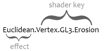
In the above example, I placed the shader stage in the second token and the API version in the third token. You aren’t required to arrange your shader keys in this way. The only requirement is that the first token corresponds to the effect file. You don’t need to use the GL3 notation for your version tokens either; in fact, you don’t have to include a version token at all. The onus is on you to create a consistent hierarchy and naming convention.
Simple Example
Here’s a text file called Blit.glsl:
-- Vertex

in vec4 Position;
void main() {
    gl_Position = Position;
}

-- Fragment

uniform sampler2D Sampler;
out vec4 FragColor;
void main() {
    ivec2 coord = ivec2(gl_FragCoord.xy);
    FragColor = texelFetch(Sampler, coord, 0);
}
Here’s how you’d use GLSW to pluck out strings from the preceding file and automatically prepend them with #line:
glswInit();
glswSetPath("./", ".glsl");
const char* vs = glswGetShader("Blit.Vertex");
const char* fs = glswGetShader("Blit.Fragment");
// ... use vs and gs here ...
glswShutdown();
GLSW does all the file I/O for you; it takes the first token from the effect key that you pass to glswGetShader, then checks if it has the effect cached; if not, it finds a file by decorating the effect name with a path prefix (in this case, “./”) and a path suffix (in this case, “.glsl”).
Ignored Text
If a section divider in your effect file does not contain any alphanumeric characters, then all text is ignored until the next section divider (or the end of the file). Also, any text that precedes the first section divider is ignored (this could be useful for a copyright notice).
If a section divider does declare a legal shader key (i.e., the first contiguous sequence of alphanumeric characters and periods), then any characters appearing before and after the shader key are ignored.
For example, the following is a silly but valid effect file:
______  _  _  _
| ___ \| |(_)| |
| |_/ /| | _ | |_
| ___ \| || || __|
| |_/ /| || || |_
\____/ |_||_| \__|

-------- Vertex --------

in vec4 Position;
void main() {
    gl_Position = Position;
}

--- /\/\/\/\/\/\/\/\ ---

Contrariwise, if it was so, it might be; and if it were so,
it would be; but as it isn't, it ain't. That's logic.

--[[[[[ Fragment <== Brigadier Lethbridge-Stewart

uniform sampler2D Sampler;
out vec4 FragColor;
void main() {
    ivec2 coord = ivec2(gl_FragCoord.xy);
    FragColor = texelFetch(Sampler, coord, 0);
}
Error Handling and Shader Key Matching
GLSW never aborts or throws exceptions. It returns 0 on failure and lets you fetch the most recent error string using glswGetError. This can happen if it can’t find the file for your specified effect key, or if you forget to call glswInit.
When GLSW tries to find a shader key that matches with the effect key requested from your C/C++ code, it doesn’t necessarily need to find an exact match. Instead, it finds the longest shader key that matches with the beginning of your requested effect key. For example, consider an effect file called TimeMachine.glsl that looks like this:
-- Vertex
FOO
-- Geometry
BAR
-- Fragment.Erosion
BAZ
-- Fragment.Grassfire
QUX
-- TessControl
QUUX
-- TessEvaluation
QUUUX
If your C++ code does this:
void test(const char* effectKey)
{
    const char* shader = glswGetShader(effectKey);
    if (shader)
        cout << shader << endl;
    else
        cout << glswGetError() << endl;
}

void main()
{
    glswInit();
    glswSetPath("", ".glsl");
    test("TimeMachine.Vertex.Grassfire");
    test("TimeMachine.Fragment.Grassfire");
    test("TimeMachine.Fragment.Cilantro");
    test("Madrid");
    glswShutdown();
}
Then your output would be this:
FOO
QUX
Could not find shader with key 'TimeMachine.Fragment.Cilantro'.
Unable to open effect file 'Madrid.glsl'.
Note that the first requested effect key did not report an error even though that exact shader key does not exist in the effect file. Here’s an example where this is useful: you’d like to use the same vertex shader with two different fragment shaders, but your rendering engine forms the string for effect keys in a generic way. For example, maybe your rendering engine defines a function that looks like this:
GLuint BuildProgram(const char* effectVariant)
{
    // ...snip...

    sprintf(effectKey, "TimeMachine.Vertex.%s", effectVariant);
    const char* vs = glswGetShader(effectKey);

    sprintf(effectKey, "TimeMachine.Fragment.%s", effectVariant);
    const char* fs = glswGetShader(effectKey);

    // ...snip...
}
If you want to use the grassfire variant of the TimeMachine effect, you’d call BuildProgram(“Grassfire”). Even though the vertex shader happens to be the same for all variants of the TimeMachine effect, the rendering engine doesn’t need to know. GLSW will simply return the longest vertex shader that matches with the beginning of “TimeMachine.Vertex.Grassfire”. This avoids complicating the file format with support for cross-referencing.
Directive Mapping
This is the only function we haven’t explained yet:
int glswAddDirectiveToken(const char* token, const char* directive);
This tells GLSW to add a token-to-directive mapping. Whenever it sees a shader key that contains the specified token, it prepends the specified directive to the top of the shader. If the specified token is an empty string, then the specified directive is prepended to all shaders. For example, given this C/C++ code:
glswInit();
glswSetPath("./", ".glsl");
glswAddDirectiveToken("", "#define FOO 1");
glswAddDirectiveToken("GL32", "#version 140");
glswAddDirectiveToken("iPhone", "#extension GL_OES_standard_derivatives : enable");

string effectKey;

effectKey = "Blit.ES2.iPhone.Fragment";
cout << effectKey << ':' << endl
     << glswGetShader(effectKey.c_str()) << endl << endl;

effectKey = "Blit.GL32.Fragment";
cout << effectKey ':' << endl
     << glswGetShader(effectKey.c_str()) << endl << endl;

glswShutdown();
You’d get output like this:
Blit.ES2.iPhone.Fragment:
#define FOO 1
#extension GL_OES_standard_derivatives : enable
#line 7
void main() {}

Blit.GL32.Fragment:
#define FOO 1
#version 140
#line 51
void main() {}
You can also use an effect name for the token parameter in glswAddDirectiveToken, which tells GLSW to prepend the specified directive to all shaders in that effect.
C’est tout!
Download
You can download GLSW as a zip file:
Or, you can download the files separately:
Lua as an Effect File Format

If you’re an OpenGL developer, you might find yourself pining for an effect file format. You’d like a standard way of specifying shader strings, but without creating a kazillion little files for all your shaders.
There aren’t many alternatives. You’re faced with such tantalizing possibilities as:
- Learn COLLADA and get mired in a Turing tarpit of entangled cross-referencing and XML namespacing.
- Travel back in time to stop Khronos from abandoning their glFX effort.
- Find someone’s made-from-scratch solution, then discover that it’s hopelessly outdated.
In this post, we’ll explore the idea of using Lua as an effect file format. We can live without some of the features that we’d expect in a more full-blown FX format (for example, having the ability to associate an effect with a specific blend or cull state). In a way, we’re simply using Lua as an organization tool for shaders.
Let’s try designating each Lua file as a single “effect”, which we’ll loosely define as “a bundle of shaders”. Usually an effect declares at least one string for each programmable stage in the OpenGL pipeline. Later in the article, we’ll group together shaders for various generations of OpenGL; this is convenient for applications that detect the platform’s capabilities at run-time.
Here’s an obvious approach to specifying an effect with Lua (note how nicely Lua handles multi-line strings):
-- Vertex Shader
MyVertexShader = [[
in vec4 Position;
uniform mat4 Projection;
void main()
{
    gl_Position = Projection * Position;
}]]

-- Fragment Shader
MyFragmentShader = [[
out vec4 FragColor;
uniform vec4 FillColor;
void main()
{
    FragColor = FillColor;
}]]
Then, in your C/C++ code, you can do something like this:
lua_State* L = lua_open();
luaL_dofile(L, "MyEffect.lua");
lua_getglobal(L, "MyVertexShader");
lua_getglobal(L, "MyFragmentShader");
const char* vs_text = lua_tostring(L, -2);
const char* fs_text = lua_tostring(L, -1);
lua_pop(L, 2);
glShaderSource(vs_handle, 1, &vs_text, 0);
glShaderSource(fs_handle, 1, &fs_text, 0);
Obviously you’d want to hide code like this behind a utility function or class method. Also, you should always check the return value from luaL_dofile. The code in this article is for illustrative purposes only.
Fixing up the Line Numbers
The problem with the above approach is that any error reporting from the shader compiler will have incorrect line numbers. In the preceding example, if the shader compiler reports an issue with line 1 of the fragment shader, then the relevant line is actually line 12 of the Lua file.
We can fix this using the #line directive in GLSL and the debug.getinfo function in Lua. Instead of declaring strings directly, we’ll need the Lua script to call a function. We can define this function in a separate file called ShaderFactory.lua:
-- Shader Factory
function DeclareShader(name, source)
    local lineNumber = debug.getinfo(2).currentline
    preamble = "#line " .. lineNumber .. "\n"
    _G[name] = preamble .. source
end
Cool usage of the _G table eh? It’s Lua’s built-in table for globals. Now our effect file becomes:
-- Vertex Shader
DeclareShader('MyVertexShader', [[
in vec4 Position;
uniform mat4 Projection;
void main()
{
    gl_Position = Projection * Position;
}]])

-- Fragment Shader
DeclareShader('MyFragmentShader', [[
out vec4 FragColor;
uniform vec4 FillColor;
void main()
{
    FragColor = FillColor;
}]])
On the C/C++ side of things, we can load in the strings just as we did before, except that our script’s usage of debug.getinfo means that we should load in Lua’s debugging library before anything else. I usually load all the utility libraries in one fell swoop using luaL_openlibs. So, our C/C++ code now looks like this:
// Create the Lua context:
lua_State* L = lua_open();

// Open Lua's utility libraries, including the debug library:
luaL_openlibs(L);

// Run the script that defines the DeclareShader function:
luaL_dofile(L, "ShaderFactory.lua");

// Load in the effect files:
luaL_dofile(L, "BrilligEffect.lua");
luaL_dofile(L, "SlithyEffect.lua");
luaL_dofile(L, "ToveEffect.lua");

// As before, extract strings and use them:
lua_getglobal(L, "MyVertexShader");
lua_getglobal(L, "MyFragmentShader");
...
Accommodating Multiple Versions of GLSL
#line isn’t the only directive we’re interested in. One of the great annoyances of OpenGL 3.0+ is the #version directive, which is required if you’d like to use the latest and greatest GLSL syntax. Ideally our DeclareShader function would somehow know if a given shader is from the OpenGL 2.0 era or the OpenGL 3.0+ era, and prepend the string accordingly. One idea is passing in the version number as an argument to the DeclareShader function, like this:
-- Shader Factory
function DeclareShader(name, version, source)
    local lineNumber = debug.getinfo(2).currentline
    preamble = "#line " .. lineNumber .. "\n" ..
               "#version " .. version .. "\n"
    _G[name] = preamble .. source
end
Although the above example is a simple solution, it’s not always good enough. Consider a situation where you need to declare multiple versions of the same shader:
-- Vertex Shader for OpenGL 3.0
DeclareShader('MyVertexShader', 130, [[
in vec4 Position;
uniform mat4 Projection;
void main()
{
    gl_Position = Projection * Position;
}]])

-- Vertex Shader for OpenGL 2.0
DeclareShader('MyVertexShader', 120, [[
void main()
{
    gl_Position = ftransform();
}]])
Unfortunately, the second call to DeclareShader will overwrite the first call. Also note that the version of the shading language itself isn’t the same as the OpenGL API. The shading language for OpenGL 2.0+ is version 120, and the shading language for 3.0+ is 130.
Ok, so we need to scope the shader names to prevent naming collisions, plus it might be nice to have DeclareShader automatically infer the language version from the API version number. Lua’s tables are great for organizing strings. The ShaderFactory.lua file now becomes:
VertexShaders = { GL2 = {}, GL3 = {}, GL4 = {}, ES2 = {} }
GeometryShaders = { GL3 = {}, GL4 = {} }
FragmentShaders = { GL2 = {}, GL3 = {}, GL4 = {}, ES2 = {} }
TessControlShaders = { GL4 = {} }
TessEvaluationShaders = { GL4 = {} }
ApiVersionToLanguageVersion = { GL2 = 120, GL3 = 130, GL4 = 150 }

function DeclareShader(stage, apiVersion, techniqueName, source)
    local tableName = stage .. "Shaders"
    local languageVersion = ApiVersionToLanguageVersion[apiVersion]
    local lineNumber = debug.getinfo(2).currentline
    _G[tableName][apiVersion][techniqueName] =
        '#version ' .. languageVersion .. '\n' ..
        '#line ' .. lineNumber .. '\n' .. source
end
Shaders for multiple versions of OpenGL can now be bundled into a single file:
-- Vertex Shader for OpenGL 2.0
DeclareShader('Vertex', 'GL2', 'SnazzyEffect', [[
void main() { /* FOO */ }
]])

-- Vertex Shader for OpenGL 3.0
DeclareShader('Vertex', 'GL3', 'SnazzyEffect', [[
void main() { /* BAR */ }
]])
Now that our shaders are hidden inside nested Lua tables, it’s a bit more footwork to access them from the C/C++ side, but we can hide the footwork behind a nice utility function like this:
const char* GetShaderSource(lua_State* L, const char* techniqueName,
                            const char* apiVersion, const char* shaderStage)
{
    // Append "Shaders" to the shader stage to obtain the table name:
    char tableName[32];
    strncpy(tableName, shaderStage, 24);
    strncat(tableName, "Shaders", 7);

    // Fetch the table from the Lua context and make sure it exists:
    lua_getglobal(L, tableName);
    if (!lua_istable(L, -1))
        return 0;

    // Make sure a table exists for the given API version:
    lua_pushstring(L, apiVersion);
    lua_gettable(L, -2);
    if (!lua_istable(L, -1))
        return 0;

    // Fetch the shader string:
    lua_pushstring(L, techniqueName);
    lua_gettable(L, -2);
    const char* shaderSource = lua_tostring(L, -1);

    // Clean up the Lua stack and return the string:
    lua_pop(L, 3);
    return shaderSource;
}
A Generalized and Terse Solution
Revisiting the Lua file, note that the shader declaration is still a bit more verbose than a dedicated effect language would be:
DeclareShader('Vertex', 'GL2', 'SnazzyEffect', 'void main() {}')
It might be nice to have Lua do some string parsing for us. Dot separators make for a nice, terse syntax. This is preferable:
DeclareShader('Vertex.GL2.SnazzyEffect', 'void main() {}')
Let’s call these dot-seperated strings shader keys. Couple more observations:
- Since we’ve deemed that each effect corresponds to a single Lua file, we can infer the effect name from the filename of the script itself.
- Instead of pre-declaring a bunch of Lua tables in ShaderFactory.lua for each programmable stage, we can create the tables dynamically.
Okay, so here’s our final version of ShaderFactory.lua:
ApiVersionToLanguageVersion = { GL2 = 120, GL3 = 140, GL4 = 150 }

function DeclareShader(shaderKey, shaderSource)

    -- Prepend the line number directive for proper error messages.
	local lineNumber = debug.getinfo(2).currentline
    shaderSource = "#line " .. lineNumber .. "\n" .. shaderSource

    -- Extract the technique name from the fullpath of the Lua script.
    local fullpath = debug.getinfo(2).source
    local f, l, technique = string.find(fullpath, "([A-Za-z]+)%.lua")

    -- If a table for this technique does not exist, create it.
    if _G[technique] == nil then
        _G[technique] = {}
    end

    -- Make sure this shader hasn't already been declared.
    if _G[technique][shaderKey] then
        error("Shader '" .. shaderKey .. "' has been declared twice.")
    end

    -- Check if an API version is in the shader key and prepend #version.
    local pos = 0
    repeat
        dummy, pos, token = string.find(shaderKey, "([A-Za-z0-9]+)", pos + 1)
        if token and ApiVersionToLanguageVersion[token] then
        	local langVersion = ApiVersionToLanguageVersion[token]
            shaderSource = "#version " .. langVersion .. "\n" .. shaderSource
        end
    until token == nil

    -- Add the shader to Lua's globals.
    _G[technique][shaderKey] = shaderSource

end
Now your effect file can look something like this:
------------ Vertex Shader for OpenGL 3.0 ------------

DeclareShader('Vertex.GL3.Erosion', [[
in vec4 Position;
void main()
{
    gl_Position = Position;
}
]])

------------ Fragment Shaders for OpenGL 3.0 ------------

DeclareShader('Fragment.GL3.Erosion.Kirk', [[
out vec4 FragColor;
void main()
{
    // ...snip...
}
]])

DeclareShader('Fragment.GL3.Erosion.Spock', [[
out vec4 FragColor;
void main()
{
    // ...snip...
}
]])
The above effect contains two fragment shaders but only one vertex shader. You’ll often find that the same vertex shader can be used for multiple fragment shaders, which is why COLLADA and the D3D FX format have so much cross-referencing. Our solution is a bit more simple: we’ll have our C/C++ utility function simply find the shader that has the longest matching shader key. You’ll see what I mean after an example.
Let’s define another term before listing out the new C/C++ utility function: an effect key is like a shader key, except that it has the effect name prepended.
const char* GetShaderSource(lua_State* L, const char* effectKey)
{
    // Extract the effect name:
    const char* targetKey = strchr(effectKey, '.');
    if (!targetKey++)
        return 0;

    char effectName[32] = {0};
    strncpy(effectName, effectKey, targetKey - effectKey - 1);

    // Fetch the table from the Lua context and make sure it exists:
    lua_getglobal(L, effectName);
    if (!lua_istable(L, -1))
    {
        lua_pop(L, 1);

        // Delay-load the Lua file:
        char effectPath[64];
        sprintf(effectPath, "%s.lua", effectName);
        if (luaL_dofile(L, effectPath))
            return 0;

        // If it's still not there, give up!
        lua_getglobal(L, effectName);
        if (!lua_istable(L, -1))
            exit(1);
    }

    const char* closestMatch = 0;
    int closestMatchLength = 0;

    int i = lua_gettop(L);
    lua_pushnil(L);
    while (lua_next(L, i) != 0)
    {
        const char* shaderKey = lua_tostring(L, -2);
        int shaderKeyLength = strlen(shaderKey);

        // Find the longest key that matches the beginning of the target key:
        if (strstr(targetKey, shaderKey) != 0 && shaderKeyLength > closestMatchLength)
        {
            closestMatchLength = shaderKeyLength;
            closestMatch = lua_tostring(L, -1);
        }

        lua_pop(L, 1);
    }

    lua_pop(L, 1);

    return closestMatch;
}
We can use the above utility function like this:
void main()
{
    lua_State* L = lua_open();
    luaL_openlibs(L);
    luaL_dofile(L, "ShaderFactory.lua");

    cout << GetShaderSource(L, "MyEffect.Vertex.GL3.Kirk") << endl << endl;
    cout << GetShaderSource(L, "MyEffect.Fragment.GL3.Kirk") << endl << endl;

    lua_close(L);
}
On line 7, the caller requests a shader from the MyEffect.lua file with a shader key of Vertex.GL3.Kirk. Since the longest matching shader key is Vertex.GL3, that’s what gets returned. Also note that the Lua script for the effect gets delay loaded.
By the way, before I let you go, let me show you a trick for commenting out big swaths of Lua code that have multi-line strings. Normally you’d use the - -[[ and - -]] delimiters for multi-line comments, but they don’t work if you’re commenting out sections that have strings delimited with [[ and ]]. Lua allows you to use alternative delimiters by inserting an arbitrary number of equal signs between the square brackets, like this:
--[==[
DeclareShader('Fragment.GL3.DisabledEffect', [[
out vec4 FragColor;
void main()
{
    // ...snip...
}
]])
--]==]

DeclareShader('Fragment.GL3.EnabledEffect', [[
out vec4 FragColor;
void main()
{
    // ...snip...
}
]])
Cool eh?