Archive for the ‘Python’ Category
Homage to Structure Synth
This post is a follow-up to something I wrote exactly one year ago: Mesh Generation with Python.
In the old post, I discussed a number of ways to generate 3D shapes in Python, and I posted some OpenGL screenshots to show off the geometry.
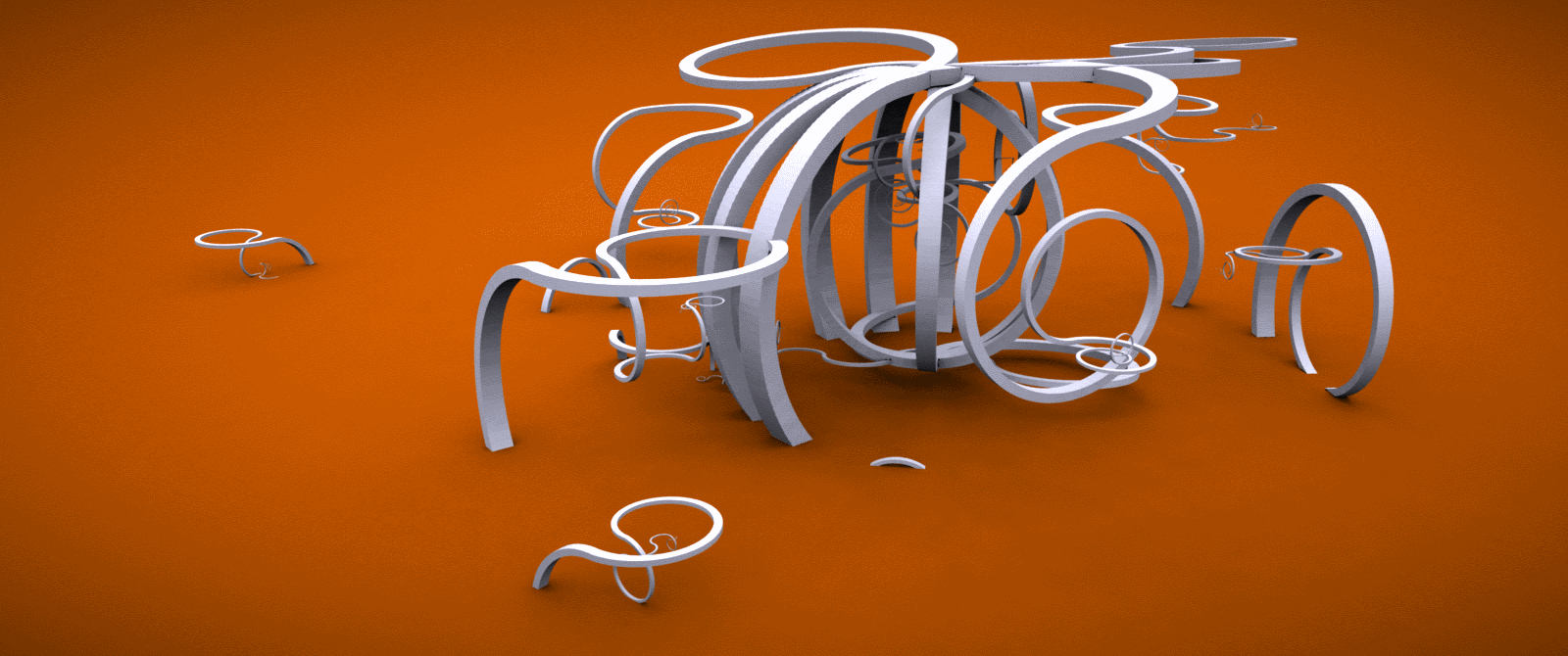
Since this is my first post since joining Pixar, I figured it would be fun to use RenderMan rather than OpenGL to show off some new procedurally-generated shapes. Sure, my new images don’t render at interactive rates, but they’re nice and high-quality:

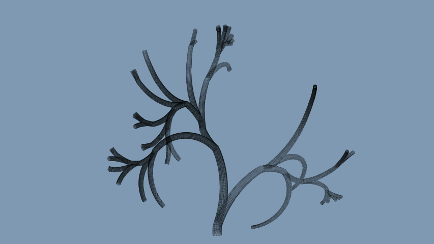
Beautiful Lindenmayer Systems
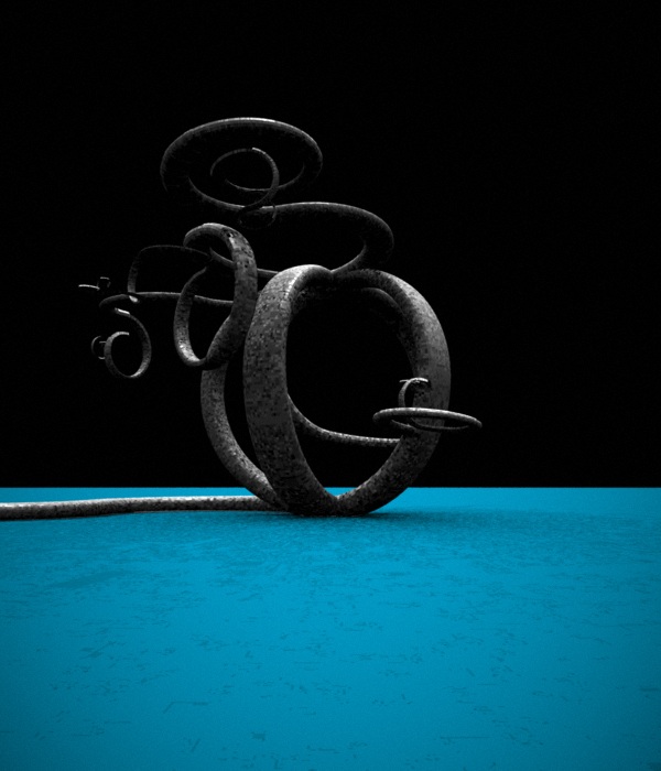
My favorite L-system from Mikael Hvidtfeldt Christensen is his Nouveau Variation; when I first saw it, I stared at it for half an hour; it’s hypnotically mathematical and surreal. He generates his art using his own software, Structure Synth.
To make similar creations without the help of Mikael’s software, I use the same XML format and Python script that I showed off in my 2010 post (here), with an extension to switch from one rule to another when a particular rule’s maximum depth is reached.
The other improvement I made was in the implementation itself; rather than using recursion to evaluate the L-system rules, I use a Python list as a stack. This turned out to simplify the code.
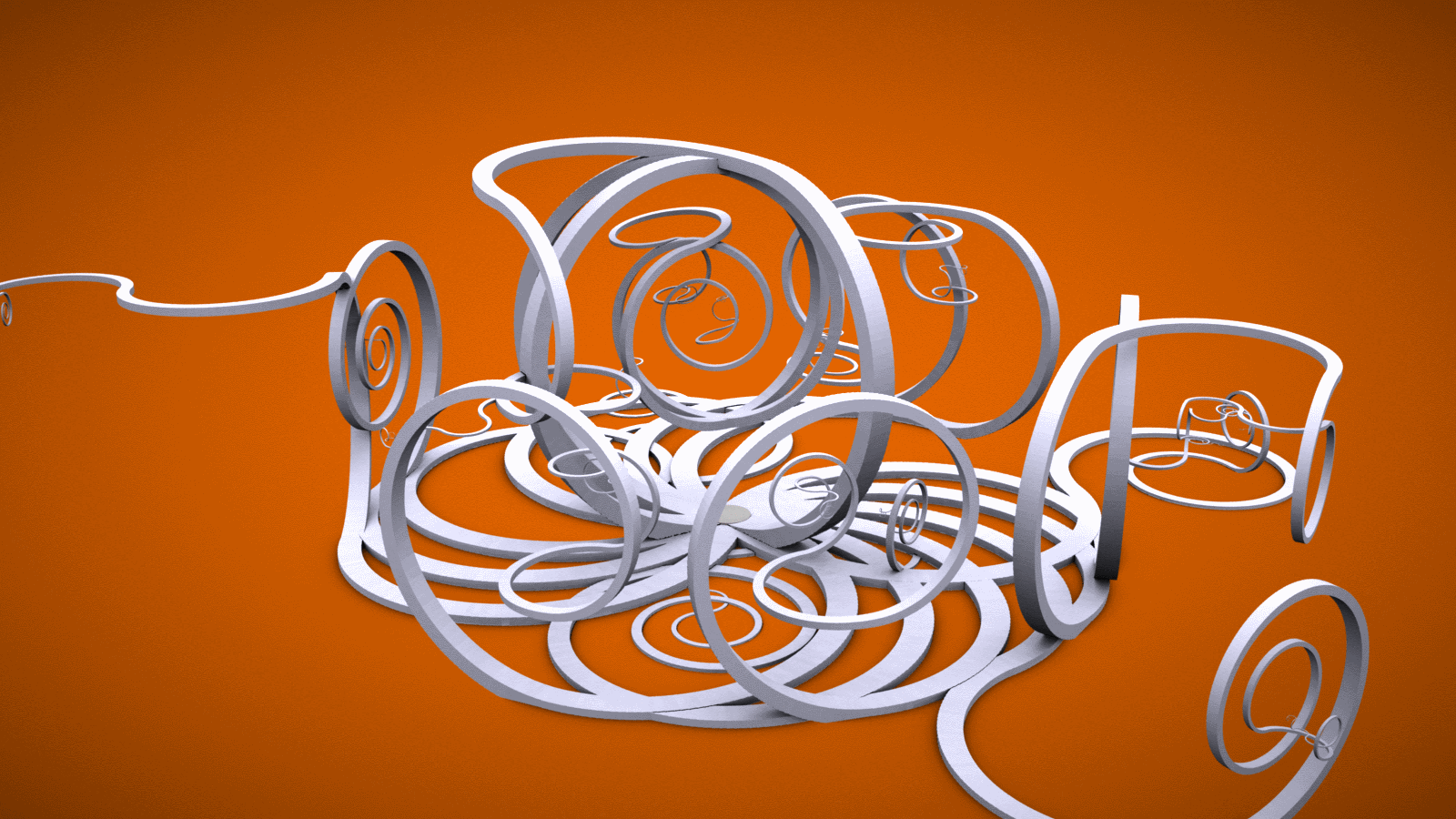
Here’s the XML representation of Mikael’s beautiful “Nouveau” L-system, which I used to generate all the images on this page:
<rules max_depth="1000">
    <rule name="entry">
        <call count="16" transforms="rz 20" rule="hbox"/>
    </rule>
    <rule name="hbox"><call rule="r"/></rule>
    <rule name="r"><call rule="forward"/></rule>
    <rule name="r"><call rule="turn"/></rule>
    <rule name="r"><call rule="turn2"/></rule>
    <rule name="r"><call rule="turn4"/></rule>
    <rule name="r"><call rule="turn3"/></rule>
    <rule name="forward" max_depth="90" successor="r">
        <call rule="dbox"/>
        <call transforms="rz 2 tx 0.1 sa 0.996" rule="forward"/>
    </rule>
    <rule name="turn" max_depth="90" successor="r">
        <call rule="dbox"/>
        <call transforms="rz 2 tx 0.1 sa 0.996" rule="turn"/>
    </rule>
    <rule name="turn2" max_depth="90" successor="r">
        <call rule="dbox"/>
        <call transforms="rz -2 tx 0.1 sa 0.996" rule="turn2"/>
    </rule>
    <rule name="turn3" max_depth="90" successor="r">
        <call rule="dbox"/>
        <call transforms="ry -2 tx 0.1 sa 0.996" rule="turn3"/>
    </rule>
    <rule name="turn4" max_depth="90" successor="r">
        <call rule="dbox"/>
        <call transforms="ry -2 tx 0.1 sa 0.996" rule="turn4"/>
    </rule>
    <rule name="turn5" max_depth="90" successor="r">
        <call rule="dbox"/>
        <call transforms="rx -2 tx 0.1 sa 0.996" rule="turn5"/>
    </rule>
    <rule name="turn6" max_depth="90" successor="r">
        <call rule="dbox"/>
        <call transforms="rx -2 tx 0.1 sa 0.996" rule="turn6"/>
    </rule>
    <rule name="dbox">
        <instance transforms="s 2.0 2.0 1.25" shape="boxy"/>
    </rule>
</rules>
Python Snippets for RenderMan
RenderMan lets you assign names to gprims, which I find useful when it reports errors. RenderMan also lets you assign gprims to various “ray groups”, which is nice when you’re using AO or Global Illumination; it lets you include/exclude certain geometry from ray-casts.
Given these two labels (an identifier and a ray group), I found it useful to extend RenderMan’s Python binding with a utility function:
def SetLabel( self, label, groups = '' ):
    """Sets the id and ray group(s) for subsequent gprims"""
    self.Attribute(self.IDENTIFIER,{self.NAME:label})
    if groups != '':
        self.Attribute("grouping",{"membership":groups})
Since Python lets you dynamically add methods to a class, you can graft the above function onto the Ri class like so:
prman.Ri.SetLabel = SetLabel
ri = prman.Ri()
# do some init stuff....
ri.SetLabel("MyHeroShape", "MovingGroup")
# instance a gprim...
I also found it useful to write some Python functions that simply called out to external processes, like the RSL compiler and the brickmap utility:
def CompileShader(shader):
    """Compiles the given RSL file"""
    print 'Compiling %s...' % shader
    retval = os.system("shader %s.sl" % shader)
    if retval:
        quit()

def CreateBrickmap(base):
    """Creates a brick map from a point cloud"""
    if os.path.exists('%s.bkm' % base):
        print "Found brickmap for %s" % base
    else:
        print "Creating brickmap for %s..." % base
        if not os.path.exists('%s.ptc' % base):
            print "Error: %s.ptc has not been generated." % base
        else:
            os.system("brickmake %s.ptc %s.bkm" % (base, base))
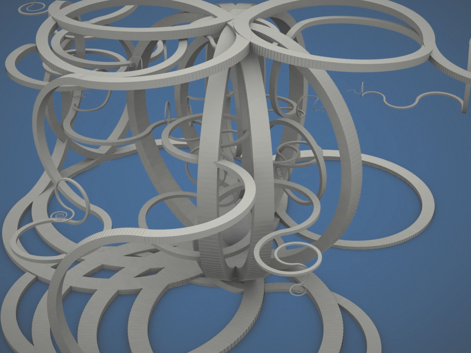
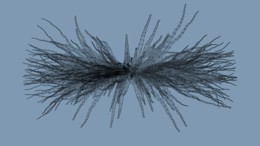
Here’s another image of the same L-system, using a different random seed:
Reminds me of Salvadore Dalí…
Some RSL Fun
The RenderMan stuff was fairly straightforward. I’m using a bog-standard AO shader:
class ComputeOcclusion(string hitgroup = "";
                       color em = (1,0,1);
                       float samples = 64)
{
  public void surface(output color Ci, Oi)
  {
    normal Nn = normalize(N);
    float occ = occlusion(P, Nn, samples,
                          "maxdist", 100.0,
                          "subset", hitgroup);

    Ci = (1 - occ) * Cs * Os;
    Ci *= em;
    Oi = Os;
  }
}
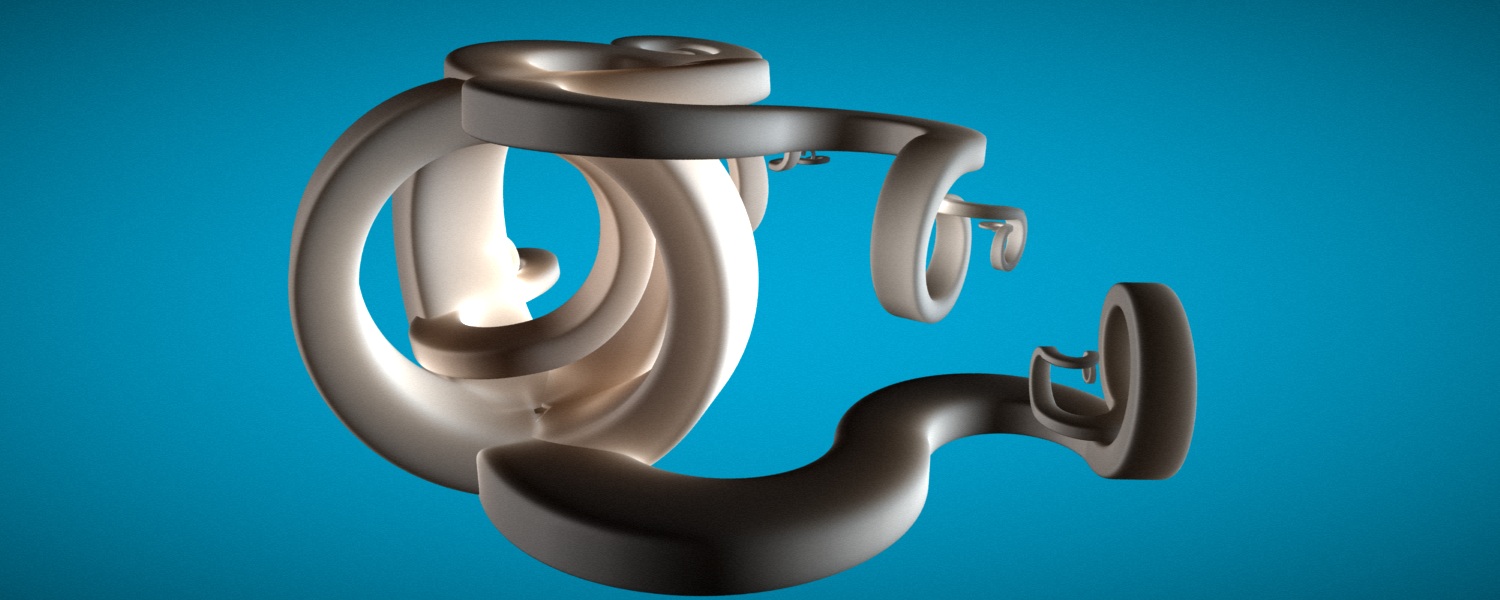
Hurray, that was my first RSL code snippet on the blog! I’m also using an imager shader to achieve the same vignette effect that Mikael used for his artwork. It just applies a radial dimming operation and adds a bit of noise to give it a photographic look:
class Vignette()
{
   public void imager(output varying color Ci; output varying color Oi)
   {
        float x = s - 0.5;
        float y = t - 0.5;
        float d = x * x + y * y;
        Ci *= 1.0 - d;

        float n = (cellnoise(s*1000, t*1000) - 0.5);
        Ci += n * 0.025;
   }
}
Downloads
Here are my Python scripts and RSL code for your enjoyment:
Gallery


Patch Surfaces and Vertex Welding
In my previous blog entry, Mesh Generation with Python, I demonstrated some techniques for generating procedural geometry, but I didn’t do much to address artistic content. Although subdivision surfaces are all the rage nowadays, bicubic patches were once considered the canonical representation of smooth surfaces. The easiest way to tesselate a bicubic patch is to evaluate it as a parametric function (not unlike the Klein bottle in my previous entry).
Back to subject of artistic content. You might be familiar with the famous Gumbo model, an Ed Catmull creation:
Turns out that Catmull originally modelled Gumbo using bicubic patches. Here’s another famous little figure that was originally modelled with patches:
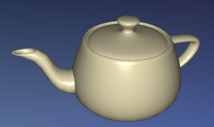
Let’s work towards the tessellation of these two classic figures, using nothing but Python and their original patch data.
Poor Man’s RIB Parser
Obviously both of these models now exist in a trillion different forms and file formats. Which one should we use in our Python sandbox? There’s one format that stands to me as a bit more authentic, at least for these two particular models. This format has been around for a while, but it’s still highly respected and in common use. Of course, I’m talking about Pixar’s RIB format.
Since we’re just playing around, we don’t need to build a robust parser for the entire RIB language; just the subset needed for these two models will suffice. Here’s an abbreviated snippet from the Gumbo rib:
TransformBegin
    Translate 7.29999 9 10
    Rotate -18 0 0 1
    Rotate -30 0 1 0
    Translate -6 0 0
    Patch "bicubic" "P" [6 0 1 ... 3 0 1]
    Patch "bicubic" "P" [6 0 2 ... 3 1 1]
    Patch "bicubic" "P" [6 1 2 ... 3 1 0]
TransformEnd
This doesn’t look too bad, especially if we have the pyeuclid module at our disposal for handling the transforms.
For parametric evaluation, the optimal representation of each patch is three 4×4 matrices: one for each XYZ axis. However, each list of numbers in the RIB file is simply a sequence of XYZ coordinates: one for each of the patch’s 16 knots (control points). We’ll give more detail on this later.
Here’s a Python function that parses a simple RIB file, tracks the current transformation matrix, and returns a set of coefficient matrices for the patches:
def create_matrices_from_rib(filename):
    file = open(filename,'r')
    coefficient_matrices = []
    transform = Matrix4()
    transform_stack = []
    for line in file:
        line = line.strip(' \t\n\r')
        tokens = re.split('[\s\[\]]', line)
        if len(tokens) < 1: continue

        action = tokens[0]
        if action == 'TransformBegin':
            transform_stack.append(transform)
        elif action == 'TransformEnd':
            transform = transform_stack[-1]
            transform_stack = transform_stack[:-1]
        elif action == 'Translate':
            xlate = map(float, tokens[1:])
            transform = transform * Matrix4.new_translate(*xlate)
        elif action == 'Scale':
            scale = map(float, tokens[1:])
            transform = transform * Matrix4.new_scale(*scale)
        elif action == 'Rotate':
            angle = float(tokens[1])
            angle = math.radians(angle)
            axis = Vector3(*map(float, tokens[2:]))
            transform = transform * Matrix4.new_rotate_axis(angle, axis)
        elif action == 'Patch':
            Cx, Cy, Cz = create_patch(tokens, transform, file)
            coefficient_matrices.append((Cx, Cy, Cz))

    return coefficient_matrices
Patch Matrices
The above snippet depends on the create_patch function to take a list of 16*3 numbers, perform some magic on them, and spit back a triplet of matrices. Here’s my implementation, and please forgive me if I’ve overdone it with the itertools module:
def create_patch(tokens, transform, file):
    """ Parse a RIB line that looks like this:
        Patch "bicubic" "P" [6 0 1 ... 3 0 1]
    """
    basis = tokens[1].strip('"')
    if basis != 'bicubic':
        print "Sorry, I only understand bicubic patches."
        quit()
    tokens = tokens[3:]

    # Parse all knots on this line:
    coords = map(float, ifilter(lambda t:len(t)>0, tokens))

    # If necessary, continue to the next line, looping until done:
    while len(coords) < 16*3:
        line = file.next()
        tokens = re.split('[\s\[\]]', line)
        c = map(float, ifilter(lambda t:len(t)>0, tokens))
        coords.extend(c)

    # Transform each knot position by the given transform:
    args = [iter(coords)] * 3
    knots = [transform * Point3(*v) for v in izip(*args)]

    # Split the coordinates into separate lists of X, Y, and Z:
    knots = [c for v in knots for c in v]
    knots = [islice(knots, n, None, 3) for n in (0,1,2)]

    # Arrange the coordinates into 4x4 matrices:
    mats = [Matrix4() for n in (0,1,2)]
    for knot, mat in izip(knots, mats):
        mat[0:16] = list(knot)

    return compute_patch_matrices(mats, bezier())
The above snippet isn’t doing anything very complex; it’s just arranging a bunch of numbers into a triplet of nice, neat 4×4 matrices. The last thing it does is call the compute_patch_matrices and bezier functions, which we’ll define shortly. This is where some math comes into play, and graphics legend Ken Perlin can explain it better than I can. Here are his course notes:
http://mrl.nyu.edu/~perlin/courses/spring2009/splines4.html
Perlin explains how you can use any of several popular matrices for your formulation, such as Hermite, Bezier, or B-Spline. We’re using Bezier:
def bezier():
    m = Matrix4()
    m[0:16] = (
        -1, 3, -3, 1,
        3, -6, 3, 0,
        -3, 3, 0, 0,
        1, 0, 0, 0 )
    return m
Here’s how we generate the three matrices from the knot positions, pretty much following Perlin’s notes verbatim:
def compute_patch_matrices(knots, B):
    assert(len(knots) == 3)
    return [B * P * B.transposed() for P in knots]
Patch Evaluation
We’ve generated a slew of coefficient matrices, but we still haven’t shown how to generate actual triangles. To do this, we’ll simply leverage the parametric evaluator from my previous post. All we need to do is supply a function object:
def make_patch_func(Cx, Cy, Cz):
    def patch(u, v):
        U = make_row_vector(u*u*u, u*u, u, 1)
        V = make_col_vector(v*v*v, v*v, v, 1)
        x = U * Cx * V
        y = U * Cy * V
        z = U * Cz * V
        return x[0], y[0], z[0]
    return patch

def load_rib(filename):

    # Parse the RIB, apply transforms, obtain a triplet of 4x4 matrices for each patch:
    knots = create_matrices_from_rib(filename)

    # Create a list of function objects that can be passed to the parametric evaluator:
    return [make_patch_func(Cx, Cy, Cz) for Cx, Cy, Cz in knots]
The pyeuclid module does not have special support for the concept of “row vectors” and “column vectors” (in fact it does not have a Vector4 type), but it’s easy enough to emulate these concepts using matrices:
def make_col_vector(a, b, c, d):
    V = Matrix4()
    V[0:16] = [a, b, c, d] + [0] * 12
    return V

def make_row_vector(a, b, c, d):
    return make_col_vector(a, b, c, d).transposed()
Here’s the final result:

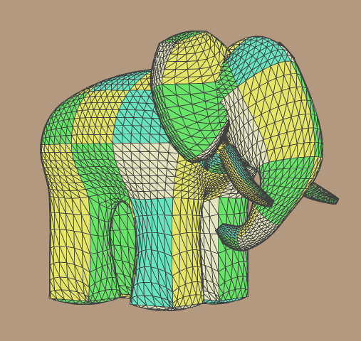
Vertex Welding
You may’ve noticed seams in the previous screenshot. The OpenCTM viewer program generates lighting normals automatically, but you shouldn’t blame it for those unsightly seams. To the viewer, those patches appear like separate surfaces. To fix this issue (and to compress the file size), we can weld the common verts along patch edges. Again, Python is a great language for expressing an algorithm like this succinctly. My implementation is by no means the fastest, but it’s good enough for me:
from math import *
from euclid import *
from itertools import *

def weld(verts, faces, epsilon = 0.00001):
    """Find duplicated verts and merge them"""

    # Create the remapping table: (this is the slow part)
    count = len(verts)
    remap_table = range(count)
    for i1 in xrange(0, count):

        # Crude progress indicator:
        if i1 % (count / 10) == 0:
            print (count - i1) / (count / 10)

        p1 = verts[i1]
        if not p1: continue

        for i2 in xrange(i1 + 1, count):
            p2 = verts[i2]
            if not p2: continue

            if abs(p1[0] - p2[0]) < epsilon and \
               abs(p1[1] - p2[1]) < epsilon and \
               abs(p1[2] - p2[2]) < epsilon:
                remap_table[i2] = i1
                verts[i2] = None

    # Remove holes from the vert list:
    newverts = []
    shift = 0
    shifts = []
    for v in xrange(count):
        if verts[v]:
            newverts.append(verts[v])
        else:
            shift = shift + 1
        shifts.append(shift)
    verts = newverts
    print "Reduced from %d verts to %d verts" % (count, len(verts))

    # Apply the remapping table:
    faces = [[x - shifts[x] for x in (remap_table[y] for y in f)] for f in faces]

    return verts, faces
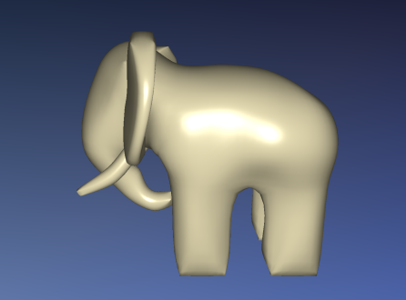
Sure enough, Gumbo’s seams disappear:
Downloads
If you want, you can download all the python scripts necessary for generating these meshes as a zip file. I also included all the stuff from my previous post in the zip.
I consider this code to be on the public domain, so don’t worry about licensing. The RIB files for the Utah Teapot and Gumbo are included.
You’ll need to download the OpenCTM SDK and the pyeuclid module from their respective sources.
Mesh Generation with Python
Do you ever find yourself needing a simple mesh for testing purposes, but you don’t want to harass your art team for the billionth time? Python is beautiful language for generating 3D mesh data. In this entry, I’ll show how to use the pyeuclid module (available on google code) combined with OpenCTM (available on sourceforge). I’ll explore various ways to generate mathematical shapes, including rule-based generation similar to Structure Synth.
Simple Example: Octohedron
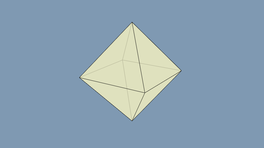
At a minimum, meshes are usually represented by two lists: a list of vertex positions (XYZ data) and a list of vertex indices (the three corners of each triangle). In Python, these are naturally represented with lists of 3-tuples. So, building an octohedron shape is easy:
from math import *

def octohedron():
    """Construct an eight-sided polyhedron"""
    f = sqrt(2.0) / 2.0
    verts = [ \
        ( 0, -1,  0),
        (-f,  0,  f),
        ( f,  0,  f),
        ( f,  0, -f),
        (-f,  0, -f),
        ( 0,  1,  0) ]
    faces = [ \
        (0, 2, 1),
        (0, 3, 2),
        (0, 4, 3),
        (0, 1, 4),
        (5, 1, 2),
        (5, 2, 3),
        (5, 3, 4),
        (5, 4, 1) ]
The tricky part is packaging up these lists into a format that OpenCTM can understand. To pull this off, we’ll need to crack our knuckles with the ctypes module. The key OpenCTM function for writing out a mesh is ctmDefineMesh, and its Python binding looks like this:
ctmDefineMesh = _lib.ctmDefineMesh
ctmDefineMesh.argtypes = [CTMcontext,
    POINTER(CTMfloat), CTMuint, # Pointer to vertex data & vertex count
    POINTER(CTMuint), CTMuint,  # Pointer to index data & triangle count
    POINTER(CTMfloat)]          # Optional pointer to surface normals
OpenCTM can represent far more than just positions and normals, but this is an easy place to get started.
So, we need to convert our Python list-of-tuples into ctypes pointers. Here’s a generic function that does just that, allowing you to pass in a custom type for the T argument (e.g., c_float):
from ctypes import *

def make_blob(verts, T):
    """Convert a list of tuples of numbers into a ctypes pointer-to-array"""
    size = len(verts) * len(verts[0])
    Blob = T * size
    floats = [c for v in verts for c in v]
    blob = Blob(*floats)
    return cast(blob, POINTER(T))
Let’s place the above code snippet into a file called blob.py and the octohedron function into a file called polyhedra.py. It’s now fairly simple to generate the mesh file:
from ctypes import *
from openctm import *
import polyhedra, blob

verts, faces = polyhedra.octohedron()
pVerts = blob.make_blob(verts, c_float)
pFaces = blob.make_blob(faces, c_uint)
pNormals = POINTER(c_float)()
ctm = ctmNewContext(CTM_EXPORT)
ctmDefineMesh(ctm, pVerts, len(verts), pFaces, len(faces), pNormals)
ctmSave(ctm, "octohedron.ctm")
ctmFreeContext(ctm)
That’s all you need to generate a simple mesh file! Note that the OpenCTM package comes with a viewer application and a conversion tool, just in case you need some other format.
Polyhedra Subdivision
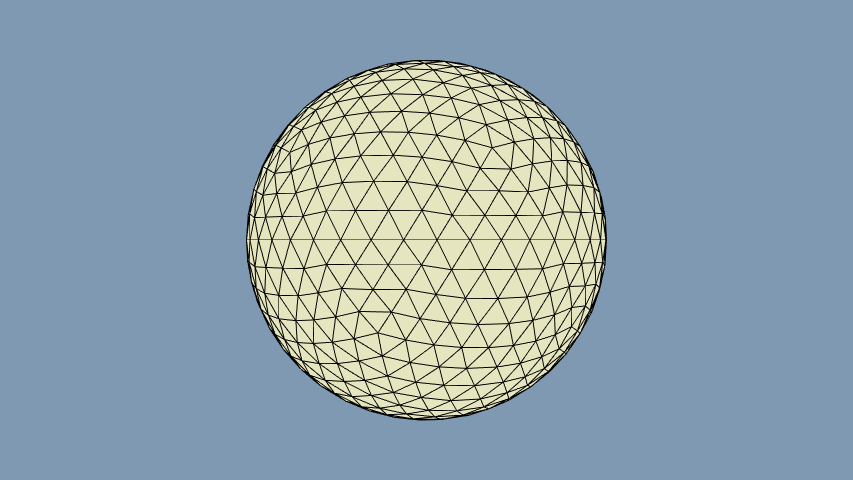
Generating a sphere is typically done by evaluating a parametric function, but if you want to avoid pole artifacts, subdividing an icosahedron produces nice results. (We’ll cover parametric functions later in the article.) Here’s a simple subdivision algorithm that uses pyeuclid for vector math. The subdivide function takes a pair of lists (verts & faces, as usual) and performs in-place subdivision, returning the modified pair of lists:
from euclid import *

def subdivide(verts, faces):
    """Subdivide each triangle into four triangles, pushing verts to the unit sphere"""
    triangles = len(faces)
    for faceIndex in xrange(triangles):

        # Create three new verts at the midpoints of each edge:
        face = faces[faceIndex]
        a,b,c = (Vector3(*verts[vertIndex]) for vertIndex in face)
        verts.append((a + b).normalized()[:])
        verts.append((b + c).normalized()[:])
        verts.append((a + c).normalized()[:])

        # Split the current triangle into four smaller triangles:
        i = len(verts) - 3
        j, k = i+1, i+2
        faces.append((i, j, k))
        faces.append((face[0], i, k))
        faces.append((i, face[1], j))
        faces[faceIndex] = (k, j, face[2])

    return verts, faces
It’s now very easy to generate a nice sphere, subdividing as many times as needed, depending on the desired level of detail:
num_subdivisions = 3
verts, faces = polyhedra.icosahedron()
for x in xrange(num_subdivisions):
    verts, faces = polyhedra.subdivide(verts, faces)

pVerts = blob.make_blob(verts, c_float)
pFaces = blob.make_blob(faces, c_uint)
# etc...
I recommend using an icosahedron as the starting point, rather than an octohedron or tetrahedron. It produces a more pleasing, symmetric geodesic pattern.
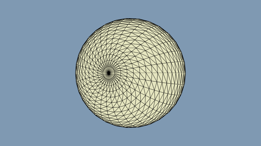
Parametric Surfaces
As promised, here’s how to generate parametric surfaces, following our existing list-of-tuples convention. The generation function takes three arguments: the level-of-detail for the U coordinate, the level-of-detail for the V coordinate, and a function object that converts the domain coordinate into a range coordinate.
from math import *

def surface(slices, stacks, func):
    verts = []
    for i in xrange(slices + 1):
        theta = i * pi / slices
        for j in xrange(stacks):
            phi = j * 2.0 * pi / stacks
            p = func(theta, phi)
            verts.append(p)

    faces = []
    v = 0
    for i in xrange(slices):
        for j in xrange(stacks):
            next = (j + 1) % stacks
            faces.append((v + j, v + next, v + j + stacks))
            faces.append((v + next, v + next + stacks, v + j + stacks))
        v = v + stacks

    return verts, faces
To use the above function, we need to pass in a function object. Of course, this can be a sphere:
def sphere(u, v):
    x = sin(u) * cos(v)
    y = cos(u)
    z = -sin(u) * sin(v)
    return x, y, z
Assuming the above two snippets are in a file called parametric.py, here’s how our top-level generation script looks:
slices, stacks = 32, 32
verts, faces = parametric.surface(slices, stacks, parametric.sphere)

pVerts = blob.make_blob(verts, c_float)
pFaces = blob.make_blob(faces, c_uint)
# etc...
A huge number of shapes can be generated by providing alternative parametric functions. Here’s a personal favorite of mine, the Klein bottle:

def klein(u, v):
    u = u * 2
    if u < pi:
        x = 3 * cos(u) * (1 + sin(u)) + (2 * (1 - cos(u) / 2)) * cos(u) * cos(v)
        z = -8 * sin(u) - 2 * (1 - cos(u) / 2) * sin(u) * cos(v)
    else:
        x = 3 * cos(u) * (1 + sin(u)) + (2 * (1 - cos(u) / 2)) * cos(v + pi)
        z = -8 * sin(u)
    y = -2 * (1 - cos(u) / 2) * sin(v)
    return x, y, z
Another type of parametric surface is a general tube shape, which brings us to the next section.
Tube Tessellation
Sometimes, all you have on hand is a simple path in 3-space; you’ve got a twisty-turny, infinitely thin length of hair, and you want to build a tube around it. The path might be supplied by an artist, or it might be generated by a mathematical function.
In another words, you’ve got list of center points for a hypothetical tube. The math for tessellating a tube is not complex, but it helps if you have the pyeuclid module at your disposal. All you need is a bit of linear algebra magic for performing a change-of-basis transformation on a plain ol’ 2D circle. Here’s a parametric function that takes a domain coordinate, a function object for the path in 3-space, and a radius:
def tube(u, v, func, radius):

    # Compute three basis vectors:
    p1 = Vector3(*func(u))
    p2 = Vector3(*func(u + 0.01))
    A = (p2 - p1).normalized()
    B = perp(A)
    C = A.cross(B).normalized()

    # Rotate the Z-plane circle appropriately:
    m = Matrix4.new_rotate_triple_axis(B, C, A)
    spoke_vector = m * Vector3(cos(2*v), sin(2*v), 0)

    # Add the spoke vector to the center to obtain the rim position:
    center = p1 + radius * spoke_vector
    return center[:]
One gotcha is the perp function, which is not part of the pyeuclid module. Every vector in 3-space has an infinite number of perpendicular vectors, so here we simply choose a random one:
def perp(u):
    """Randomly pick a reasonable perpendicular vector"""
    u_prime = u.cross(Vector3(1, 0, 0))
    if u_prime.magnitude_squared() < 0.01:
       u_prime = u.cross(v = Vector3(0, 1, 0))
    return u_prime.normalized()
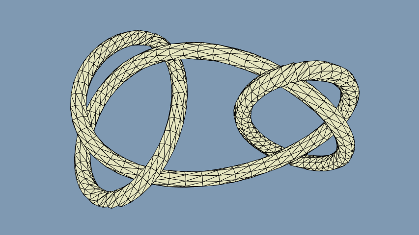
Generic tube tessellation is useful for visualizing various knot shapes. Here’s the formula for the so-called “Granny Knot” (depicted above):
def granny_path(t):
    t = 2 * t
    x = -0.22 * cos(t) - 1.28 * sin(t) - 0.44 * cos(3 * t) - 0.78 * sin(3 * t)
    y = -0.1 * cos(2 * t) - 0.27 * sin(2 * t) + 0.38 * cos(4 * t) + 0.46 * sin(4 * t)
    z = 0.7 * cos(3 * t) - 0.4 * sin(3 * t)
    return x, y, z
To tessellate the actual tube, we need to use this function in conjunction with our existing parametric surface function. Here’s how our top-level script can do so:
def granny(u, v):
    return tube(u, v, granny_path, radius = 0.1)

verts, faces = parametric.surface(slices, stacks, granny)
pVerts = make_blob(verts, c_float)
pFaces = make_blob(faces, c_uint)
# etc...
Rule-Based Generation
Rule-based generation is a cool way of generating fractal-like shapes. StructureSynth and Context Free are a couple popular packages for generating these type of meshes, but it’s actually pretty easy to write an evaluator from scratch. In this section, we’ll devise a simple XML-based format for representing the rules, and we’ll use Python to evaluate the rules and dump out a mesh.
The XML file defines a set of rules, each of which contains a list of instructions. There are only two instructions: the instance instruction, which stamps down a small predefined shape, and the call function, which calls another rule. Multiple rules can have the same name, in which case the evaluator picks a rule at random. Rules can be assigned a weight if you want to give them a higher probability of being chosen. If you don’t specify a weight, it defaults to one.
Each instruction has an associated count and an associated set of transformations. If you don’t specify a count, it defaults to 1. If you don’t specify a transformation, it defaults to an identity transformation.
Since recursion is a fundamental aspect of rule-based mesh generation, our evaluator requires you to specify a maximum call depth using the max_depth attribute in the top-level XML element.
Now, without further ado, here’s the XML description for the preceding tree shape, which is based on a Structure Synth example:
<rules max_depth="200">
    <rule name="entry">
        <call transforms="ry 180" rule="spiral"/>
    </rule>
    <rule name="spiral" weight="100">
        <instance shape="tubey"/>
        <call transforms="ty 0.4 rx 1 sa 0.995" rule="spiral"/>
    </rule>
    <rule name="spiral" weight="100">
        <instance shape="tubey"/>
        <call transforms="ty 0.4 rx 1 ry 1 sa 0.995" rule="spiral"/>
    </rule>
    <rule name="spiral" weight="100">
        <instance shape="tubey"/>
        <call transforms="ty 0.4 rx 1 rz -1 sa 0.995" rule="spiral"/>
    </rule>
    <rule name="spiral" weight="6">
        <call transforms="rx 15" rule="spiral"/>
        <call transforms="ry 180" rule="spiral"/>
    </rule>
</rules>
Every description must contain at least one rule named entry; this is the starting point for the evaluator. Note the mini-language used for specifying transformations. It’s a simple string consisting of translations, rotations, and scaling operations. For example, tx n means “translate n units along the x-axis”, ry theta means “rotate theta degrees about the y-axis”, and sa f means “scale all axes by a factor of f“.
It’s surprisingly easy to write a Python module that slurps up the preceding XML, evaluates the rules, and dumps out a mesh file. The module has only one public function: the surface function, which takes an XML string for input and returns lists of vertex positions and indices:
from math import *
from euclid import *
from lxml import etree
from lxml import objectify
import random

def surface(rules_string):
    verts, faces = [], []
    tree = objectify.fromstring(rules_string)
    max_depth = int(tree.get('max_depth'))
    entry = pick_rule(tree, "entry")
    process_rule(entry, tree, max_depth, verts, faces)
    print "nverts, nfaces = ", len(verts), len(faces)
    return verts, faces
The module defines three private functions:
- pick_rule
-
Takes the entire DOM and a string name for input; chooses a random rule with the given name, respecting the weights. Returns the XML element for the chosen rule.
- parse_transform
-
Parses a transformation string and returns the resulting matrix.
- process_rule
-
The key function in the evaluator. Takes an XML element for a specific rule to evaluate and a transformation matrix. Contains a loop to respect the count attribute, and calls itself as needed.
To see the source code for these functions, check out the downloads section.
Before finishing up the blog entry, let me leave you with another cool rule-based shape inspired by a Structure Synth example:
The XML for this is pretty simple:
<rules max_depth="20">
    <rule name="entry">
        <call count="300" transforms="ry 3.6" rule="arm"/>
    </rule>
    <rule name="arm">
        <call transforms="sa 0.9 rz 6 tx 1" rule="arm"/>
        <instance transforms="s 1 0.2 0.5" shape="box"/>
    </rule>
    <rule name="arm">
        <call transforms="sa 0.9 rz -6 tx 1" rule="arm"/>
        <instance transforms="s 1 0.2 0.5" shape="box"/>
    </rule>
</rules>
Downloads
If you want, you can download all the python scripts necessary for generating these meshes as a zip file. I consider this code to be on the public domain, so don’t worry about licensing.
You’ll need to download the OpenCTM SDK and the pyeuclid module from their respective sources.
“iPhone 3D” In Stock At Amazon!
Amazon has replaced the Pre-order button for my book with Add to Cart. To celebrate, I created a word cloud of the entire book using wordle.net and a python script. Here’s the word cloud:
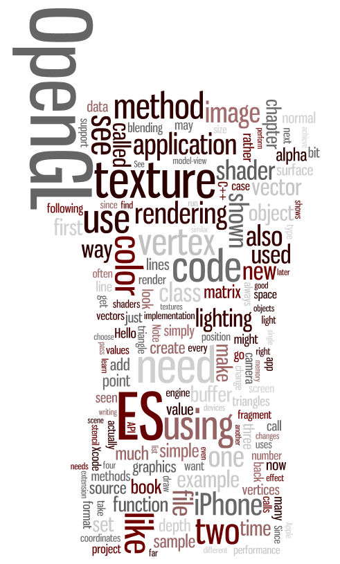
I love that “API” got nestled into “ES”. To create the word cloud, I first ran a little python script against the book’s DocBook source. The script simply extracts content from para elements. If I don’t do this, the word cloud contains all the sample code and represents words like const in huge, overwhelming text. (I tried it, trust me.) Anyway here’s the script:
from xml.dom.minidom import parse
import codecs

def getText(nodelist):
    rc = ""
    for node in nodelist:
        if node.nodeType == node.TEXT_NODE:
            rc = rc + node.data
    return rc

f = codecs.open( "wordle.txt", "w", "utf-8" )

for i in xrange(0, 10):
    filename = "ch%02d.xml" % i
    tree = parse(filename)
    paras = tree.getElementsByTagName("para")
    for para in paras:
        f.write(getText(para.childNodes))

print "wordle.txt has been dumped"
After running the script, I simply pasted the resulting text file into wordle.net.