In my previous blog entry, Mesh Generation with Python, I demonstrated some techniques for generating procedural geometry, but I didn’t do much to address artistic content. Although subdivision surfaces are all the rage nowadays, bicubic patches were once considered the canonical representation of smooth surfaces. The easiest way to tesselate a bicubic patch is to evaluate it as a parametric function (not unlike the Klein bottle in my previous entry).

Back to subject of artistic content. You might be familiar with the famous Gumbo model, an Ed Catmull creation:

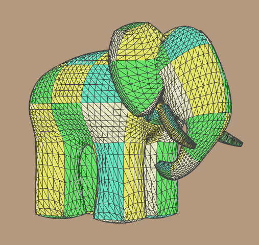
Turns out that Catmull originally modelled Gumbo using bicubic patches. Here’s another famous little figure that was originally modelled with patches:

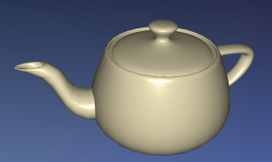
Let’s work towards the tessellation of these two classic figures, using nothing but Python and their original patch data.

Poor Man’s RIB Parser

Obviously both of these models now exist in a trillion different forms and file formats. Which one should we use in our Python sandbox? There’s one format that stands to me as a bit more authentic, at least for these two particular models. This format has been around for a while, but it’s still highly respected and in common use. Of course, I’m talking about Pixar’s RIB format.

Since we’re just playing around, we don’t need to build a robust parser for the entire RIB language; just the subset needed for these two models will suffice. Here’s an abbreviated snippet from the Gumbo rib:

TransformBegin 
    Translate 7.29999 9 10
    Rotate -18 0 0 1
    Rotate -30 0 1 0
    Translate -6 0 0
    Patch "bicubic" "P" [6 0 1 ... 3 0 1]
    Patch "bicubic" "P" [6 0 2 ... 3 1 1]
    Patch "bicubic" "P" [6 1 2 ... 3 1 0]
TransformEnd 

This doesn’t look too bad, especially if we have the pyeuclid module at our disposal for handling the transforms.

For parametric evaluation, the optimal representation of each patch is three 4×4 matrices: one for each XYZ axis. However, each list of numbers in the RIB file is simply a sequence of XYZ coordinates: one for each of the patch’s 16 knots (control points). We’ll give more detail on this later.

Here’s a Python function that parses a simple RIB file, tracks the current transformation matrix, and returns a set of coefficient matrices for the patches:

def create_matrices_from_rib(filename):
    file = open(filename,'r') 
    coefficient_matrices = []
    transform = Matrix4()
    transform_stack = []
    for line in file:
        line = line.strip(' \t\n\r')
        tokens = re.split('[\s\[\]]', line)
        if len(tokens) < 1: continue
            
        action = tokens[0]
        if action == 'TransformBegin':
            transform_stack.append(transform)
        elif action == 'TransformEnd':
            transform = transform_stack[-1]
            transform_stack = transform_stack[:-1]
        elif action == 'Translate':
            xlate = map(float, tokens[1:])
            transform = transform * Matrix4.new_translate(*xlate)
        elif action == 'Scale':
            scale = map(float, tokens[1:])
            transform = transform * Matrix4.new_scale(*scale)
        elif action == 'Rotate':
            angle = float(tokens[1])
            angle = math.radians(angle)
            axis = Vector3(*map(float, tokens[2:]))
            transform = transform * Matrix4.new_rotate_axis(angle, axis)
        elif action == 'Patch':
            Cx, Cy, Cz = create_patch(tokens, transform, file)
            coefficient_matrices.append((Cx, Cy, Cz))
            
    return coefficient_matrices

Patch Matrices

The above snippet depends on the create_patch function to take a list of 16*3 numbers, perform some magic on them, and spit back a triplet of matrices. Here’s my implementation, and please forgive me if I’ve overdone it with the itertools module:

def create_patch(tokens, transform, file):
    """ Parse a RIB line that looks like this:
        Patch "bicubic" "P" [6 0 1 ... 3 0 1]
    """
    basis = tokens[1].strip('"')
    if basis != 'bicubic':
        print "Sorry, I only understand bicubic patches."
        quit()
    tokens = tokens[3:]
    
    # Parse all knots on this line:
    coords = map(float, ifilter(lambda t:len(t)>0, tokens))
            
    # If necessary, continue to the next line, looping until done:
    while len(coords) < 16*3:
        line = file.next()
        tokens = re.split('[\s\[\]]', line)
        c = map(float, ifilter(lambda t:len(t)>0, tokens))
        coords.extend(c)

    # Transform each knot position by the given transform:
    args = [iter(coords)] * 3
    knots = [transform * Point3(*v) for v in izip(*args)]

    # Split the coordinates into separate lists of X, Y, and Z:
    knots = [c for v in knots for c in v]
    knots = [islice(knots, n, None, 3) for n in (0,1,2)]

    # Arrange the coordinates into 4x4 matrices:
    mats = [Matrix4() for n in (0,1,2)]
    for knot, mat in izip(knots, mats):
        mat[0:16] = list(knot)
    
    return compute_patch_matrices(mats, bezier())

The above snippet isn’t doing anything very complex; it’s just arranging a bunch of numbers into a triplet of nice, neat 4×4 matrices. The last thing it does is call the compute_patch_matrices and bezier functions, which we’ll define shortly. This is where some math comes into play, and graphics legend Ken Perlin can explain it better than I can. Here are his course notes:

http://mrl.nyu.edu/~perlin/courses/spring2009/splines4.html

Perlin explains how you can use any of several popular matrices for your formulation, such as Hermite, Bezier, or B-Spline. We’re using Bezier:

def bezier():
    m = Matrix4()
    m[0:16] = (
        -1, 3, -3, 1,
        3, -6, 3, 0,
        -3, 3, 0, 0,
        1, 0, 0, 0 )
    return m

Here’s how we generate the three matrices from the knot positions, pretty much following Perlin’s notes verbatim:

def compute_patch_matrices(knots, B):
    assert(len(knots) == 3)
    return [B * P * B.transposed() for P in knots]

Patch Evaluation

We’ve generated a slew of coefficient matrices, but we still haven’t shown how to generate actual triangles. To do this, we’ll simply leverage the parametric evaluator from my previous post. All we need to do is supply a function object:

def make_patch_func(Cx, Cy, Cz):
    def patch(u, v):
        U = make_row_vector(u*u*u, u*u, u, 1)
        V = make_col_vector(v*v*v, v*v, v, 1)
        x = U * Cx * V
        y = U * Cy * V
        z = U * Cz * V
        return x[0], y[0], z[0]
    return patch

def load_rib(filename):
    
    # Parse the RIB, apply transforms, obtain a triplet of 4x4 matrices for each patch:
    knots = create_matrices_from_rib(filename)
    
    # Create a list of function objects that can be passed to the parametric evaluator:
    return [make_patch_func(Cx, Cy, Cz) for Cx, Cy, Cz in knots]

The pyeuclid module does not have special support for the concept of “row vectors” and “column vectors” (in fact it does not have a Vector4 type), but it’s easy enough to emulate these concepts using matrices:

def make_col_vector(a, b, c, d):
    V = Matrix4()
    V[0:16] = [a, b, c, d] + [0] * 12
    return V

def make_row_vector(a, b, c, d):
    return make_col_vector(a, b, c, d).transposed()

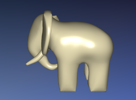
Here’s the final result:

Vertex Welding

You may’ve noticed seams in the previous screenshot. The OpenCTM viewer program generates lighting normals automatically, but you shouldn’t blame it for those unsightly seams. To the viewer, those patches appear like separate surfaces. To fix this issue (and to compress the file size), we can weld the common verts along patch edges. Again, Python is a great language for expressing an algorithm like this succinctly. My implementation is by no means the fastest, but it’s good enough for me:

from math import *
from euclid import *
from itertools import *

def weld(verts, faces, epsilon = 0.00001):
    """Find duplicated verts and merge them"""
    
    # Create the remapping table: (this is the slow part)
    count = len(verts)
    remap_table = range(count)
    for i1 in xrange(0, count):

        # Crude progress indicator:
        if i1 % (count / 10) == 0:
            print (count - i1) / (count / 10)
    
        p1 = verts[i1]
        if not p1: continue

        for i2 in xrange(i1 + 1, count):
            p2 = verts[i2]
            if not p2: continue

            if abs(p1[0] - p2[0]) < epsilon and \
               abs(p1[1] - p2[1]) < epsilon and \
               abs(p1[2] - p2[2]) < epsilon:
                remap_table[i2] = i1
                verts[i2] = None

    # Remove holes from the vert list:
    newverts = []
    shift = 0
    shifts = []
    for v in xrange(count):
        if verts[v]:
            newverts.append(verts[v])
        else:
            shift = shift + 1
        shifts.append(shift)
    verts = newverts
    print "Reduced from %d verts to %d verts" % (count, len(verts))

    # Apply the remapping table:
    faces = [[x - shifts[x] for x in (remap_table[y] for y in f)] for f in faces]

    return verts, faces

Sure enough, Gumbo’s seams disappear:

Downloads

If you want, you can download all the python scripts necessary for generating these meshes as a zip file. I also included all the stuff from my previous post in the zip.

I consider this code to be on the public domain, so don’t worry about licensing. The RIB files for the Utah Teapot and Gumbo are included.

• patches.zip

You’ll need to download the OpenCTM SDK and the pyeuclid module from their respective sources.