Archive for the ‘opengl’ tag
Single-Pass Raycasting
Raycasting over a volume requires start and stop points for your rays. The traditional method for computing these intervals is to draw a cube (with perspective) into two surfaces: one surface has front faces, the other has back faces. By using a fragment shader that writes object-space XYZ into the RGB channels, you get intervals. Your final pass is the actual raycast.
In the original incarnation of this post, I proposed making it into a single pass process by dilating a back-facing triangle from the cube and performing perspective-correct interpolation math in the fragment shader. Simon Green pointed out that this was a bit silly, since I can simply do a ray-cube intersection. So I rewrote this post, showing how to correlate a field-of-view angle (typically used to generate an OpenGL projection matrix) and focal length (typically used to determine ray direction). This might be useful to you if you need to integrate a raycast volume into an existing 3D scene that uses traditional rendering.
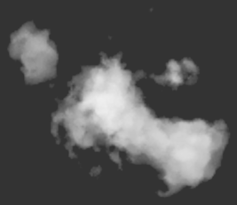
To have something interesting to render in the demo code (download is at the end of the post), I generated a pyroclastic cloud as described in this amazing PDF on volumetric methods from the 2010 SIGGRAPH course. Miles Macklin has a simply great blog entry about it here.
Recap of Two-Pass Raycasting
Here’s a depiction of the usual offscreen surfaces for ray intervals:
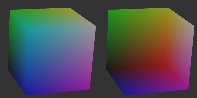
Front faces give you the start points and the back faces give you the end points. The usual procedure goes like this:
-
Draw a cube’s front faces into surface A and back faces into surface B. This determines ray intervals.
- Attach two textures to the current FBO to render to both surfaces simultaneously.
- Use a fragment shader that writes out normalized object-space coordinates to the RGB channels.
-
Draw a full-screen quad to perform the raycast.
- Bind three textures: the two interval surfaces, and the 3D texture you’re raycasting against.
- Sample the two interval surfaces to obtain ray start and stop points. If they’re equal, issue a discard.
Making it Single-Pass
To make this a one-pass process and remove two texture lookups from the fragment shader, we can use a procedure like this:
-
Draw a cube’s front-faces to perform the raycast.
- On the CPU, compute the eye position in object space and send it down as a uniform.
- Also on the CPU, compute a focal length based on the field-of-view that you’re using to generate your scene’s projection matrix.
- At the top of the fragment shader, perform a ray-cube intersection.
Raycasting on front-faces instead of a full-screen quad allows you to avoid the need to test for intersection failure. Traditional raycasting shaders issue a discard if there’s no intersection with the view volume, but since we’re guaranteed to hit the viewing volume, so there’s no need.
Without further ado, here’s my fragment shader using modern GLSL syntax:
out vec4 FragColor;

uniform mat4 Modelview;
uniform float FocalLength;
uniform vec2 WindowSize;
uniform vec3 RayOrigin;

struct Ray {
    vec3 Origin;
    vec3 Dir;
};

struct AABB {
    vec3 Min;
    vec3 Max;
};

bool IntersectBox(Ray r, AABB aabb, out float t0, out float t1)
{
    vec3 invR = 1.0 / r.Dir;
    vec3 tbot = invR * (aabb.Min-r.Origin);
    vec3 ttop = invR * (aabb.Max-r.Origin);
    vec3 tmin = min(ttop, tbot);
    vec3 tmax = max(ttop, tbot);
    vec2 t = max(tmin.xx, tmin.yz);
    t0 = max(t.x, t.y);
    t = min(tmax.xx, tmax.yz);
    t1 = min(t.x, t.y);
    return t0 <= t1;
}

void main()
{
    vec3 rayDirection;
    rayDirection.xy = 2.0 * gl_FragCoord.xy / WindowSize - 1.0;
    rayDirection.z = -FocalLength;
    rayDirection = (vec4(rayDirection, 0) * Modelview).xyz;

    Ray eye = Ray( RayOrigin, normalize(rayDirection) );
    AABB aabb = AABB(vec3(-1.0), vec3(+1.0));

    float tnear, tfar;
    IntersectBox(eye, aabb, tnear, tfar);
    if (tnear < 0.0) tnear = 0.0;

    vec3 rayStart = eye.Origin + eye.Dir * tnear;
    vec3 rayStop = eye.Origin + eye.Dir * tfar;

    // Transform from object space to texture coordinate space:
    rayStart = 0.5 * (rayStart + 1.0);
    rayStop = 0.5 * (rayStop + 1.0);

    // Perform the ray marching:
    vec3 pos = rayStart;
    vec3 step = normalize(rayStop-rayStart) * stepSize;
    float travel = distance(rayStop, rayStart);
    for (int i=0; i < MaxSamples && travel > 0.0; ++i, pos += step, travel -= stepSize) {

        // ...lighting and absorption stuff here...

    }
The shader works by using gl_FragCoord and a given FocalLength value to generate a ray direction. Just like a traditional CPU-based raytracer, the appropriate analogy is to imagine holding a square piece of chicken wire in front of you, tracing rays from your eyes through the holes in the mesh.
If you’re integrating the raycast volume into an existing scene, computing FocalLength and RayOrigin can be a little tricky, but it shouldn’t be too difficult. Here’s a little sketch I made:
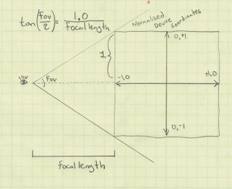
In days of yore, most OpenGL programmers would use the gluPerspective function to compute a projection matrix, although nowadays you’re probably using whatever vector math library you happen to be using. My personal favorite is the simple C++ vector library from Sony that’s included in Bullet. Anyway, you’re probably calling a function that takes a field-of-view angle as an argument:
Matrix4 Perspective(float fovy, float aspectRatio, float nearPlane, float farPlane);
Based on the above diagram, converting the fov value into a focal length is easy:
float focalLength = 1.0f / tan(FieldOfView / 2);
You’re also probably calling function kinda like gluLookAt to compute your view matrix:
Matrix4 LookAt(Point3 eyePosition, Point3 targetPosition, Vector3 up);
To compute a ray origin, transform the eye position from world space into object space, relative to the viewing cube.
Downloads
I’ve tested the code with Visual Studio 2010. It uses CMake for the build system.
I consider this code to be on the public domain. Enjoy!
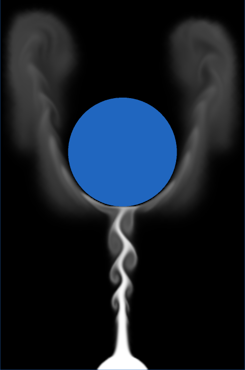
Simple Fluid Simulation
I finally wrote my first fluid simulation: two-dimensional smoke advected with GLSL fragment shaders. It was great fun, but let me warn you: it’s all too easy to drain away vast swaths of your life while tuning the millions of various parameters, just to get the right effect. It’s also rather addictive.
For my implementation, I used the classic Mark Harris article from GPU Gems 1 as my trusty guide. His article is available online here. Ah, 2004 seems like it was only yesterday…
Mark’s article is about a method called Eulerian Grid. In general, fluid simulation algorithms can be divided into three categories:
- Eulerian
-
Divides a cuboid of space into cells. Each cell contains a velocity vector and other information, such as density and temperature.
- Lagrangian
-
Particle-based physics, not as effective as Eulerian Grid for modeling “swirlies”. However, particles are much better for expansive regions, since they aren’t restricted to a grid.
- Hybrid
-
For large worlds that have specific regions where swirlies are desirable, use Lagrangian everywhere, but also place Eulerian grids in the regions of interest. When particles enter those regions, they become influenced by the grid’s velocity vectors. Jonathan Cohen has done some interesting work in this area.
Regardless of the method, the Navier-Stokes equation is at the root of it all. I won’t cover it here since you can read about it from a trillion different sources, all of which are far more authoritative than this blog. I’m focusing on implementation.
After reading Mark’s article, I found it useful to create a quick graphviz diagram for all the image processing:
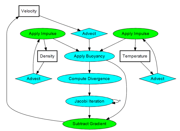
It’s not as complicated as it looks. The processing stages are all drawing full-screen quads with surprisingly simple fragment shaders. There are a total of three floating-point surfaces being processed: Velocity (a 2-component texture), Density (a 1-component texture), and Temperature (another 1-component texture).
In practice, you’ll need six surfaces instead of three; this allows ping-ponging between render targets and source textures. In some cases you can use blending instead; those stages are shown in green.
The processing stages are:
- Advect
-
Copies a quantity from a neighboring cell into the current cell; projects the current velocity backwards to find the incoming value. This is used for any type of quantity, including density, temperature, and velocity itself.
- Apply Impulse
-
This stage accounts for external forces, such as user interaction or the immortal candle in my simulation.
- Apply Buoyancy
-
For smoke effects, temperature can influence velocity by making it rise. In my implementation, I also apply the weight of the smoke in this stage; high densities in cool regions will sink.
- Compute Divergence
-
This stage computes values for a temporary surface (think of it as “scratch space”) that’s required for computing the pressure component of the Navier-Stokes equation.
- Jacobi Iteration
-
This is the real meat of the algorithm; it requires many iterations to converge to a good pressure value. The number of iterations is one of the many tweakables that I referred to at the beginning of this post, and I found that ~40 iterations was a reasonable number.
- Subtract Gradient
-
In this stage, the gradient of the pressure gets subtracted from velocity.
The above list is by no means set in stone — there are many ways to create a fluid simulation. For example, the Buoyancy stage is not necessary for liquids. Also, many simulations have a Vorticity Confinement stage to better preserve curliness, which I decided to omit. I also left out a Viscous Diffusion stage, since it’s not very useful for smoke.
Dealing with obstacles is tricky. One way of enforcing boundary conditions is adding a new operation after every processing stage. The new operation executes a special draw call that only touches the pixels that need to be tweaked to keep Navier-Stokes happy.
Alternatively, you can perform boundary enforcement within your existing fragment shaders. This adds costly texture lookups, but makes it easier to handle dynamic boundaries, and it simplifies your top-level image processing logic. Here’s the new diagram that takes obstacles into account: (alas, we can no longer use blending for SubtractGradient)
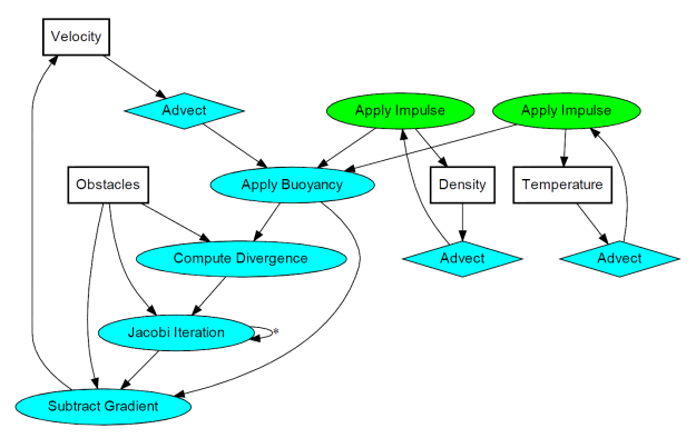
Note that I added a new surface called Obstacles. It has three components: the red component is essentially a boolean for solid versus empty, and the green/blue channels represent the obstacle’s velocity.
For my C/C++ code, I defined tiny POD structures for the various surfaces, and simple functions for each processing stage. This makes the top-level rendering routine easy to follow:
struct Surface {
    GLuint FboHandle;
    GLuint TextureHandle;
    int NumComponents;
};

struct Slab {
    Surface Ping;
    Surface Pong;
};

Slab Velocity, Density, Pressure, Temperature;
Surface Divergence, Obstacles;

// [snip]

glViewport(0, 0, GridWidth, GridHeight);

Advect(Velocity.Ping, Velocity.Ping, Obstacles, Velocity.Pong, VelocityDissipation);
SwapSurfaces(&Velocity);

Advect(Velocity.Ping, Temperature.Ping, Obstacles, Temperature.Pong, TemperatureDissipation);
SwapSurfaces(&Temperature);

Advect(Velocity.Ping, Density.Ping, Obstacles, Density.Pong, DensityDissipation);
SwapSurfaces(&Density);

ApplyBuoyancy(Velocity.Ping, Temperature.Ping, Density.Ping, Velocity.Pong);
SwapSurfaces(&Velocity);

ApplyImpulse(Temperature.Ping, ImpulsePosition, ImpulseTemperature);
ApplyImpulse(Density.Ping, ImpulsePosition, ImpulseDensity);

ComputeDivergence(Velocity.Ping, Obstacles, Divergence);
ClearSurface(Pressure.Ping, 0);

for (int i = 0; i < NumJacobiIterations; ++i) {
    Jacobi(Pressure.Ping, Divergence, Obstacles, Pressure.Pong);
    SwapSurfaces(&Pressure);
}

SubtractGradient(Velocity.Ping, Pressure.Ping, Obstacles, Velocity.Pong);
SwapSurfaces(&Velocity);
For my full source code, you can download the zip at the end of this article, but I’ll go ahead and give you a peek at the fragment shader for one of the processing stages. Like I said earlier, these shaders are mathematically simple on their own. I bet most of the performance cost is in the texture lookups, not the math. Here’s the shader for the Advect stage:
out vec4 FragColor;

uniform sampler2D VelocityTexture;
uniform sampler2D SourceTexture;
uniform sampler2D Obstacles;

uniform vec2 InverseSize;
uniform float TimeStep;
uniform float Dissipation;

void main()
{
    vec2 fragCoord = gl_FragCoord.xy;
    float solid = texture(Obstacles, InverseSize * fragCoord).x;
    if (solid > 0) {
        FragColor = vec4(0);
        return;
    }

    vec2 u = texture(VelocityTexture, InverseSize * fragCoord).xy;
    vec2 coord = InverseSize * (fragCoord - TimeStep * u);
    FragColor = Dissipation * texture(SourceTexture, coord);
}
Downloads
 The demo code uses a subset of the Pez ecosystem, which is included in the zip below. It can be built with Visual Studio 2010 or gcc. For the latter, I provided a WAF script instead of a makefile.
I consider this code to be on the public domain. Enjoy!