Robert Bridson, that esteemed guru of fluid simulation, wrote a short-n-sweet 2007 SIGGRAPH paper on using Perlin noise to create turbulent effects in a divergence-free velocity field (PDF). Divergence-free means that the velocity field conforms to the incompressibility aspect of Navier-Stokes, making it somewhat believable from a physics standpoint. It’s a nice way to fake a fluid if you don’t have enough horsepower for a more rigorous physically-based system, such as the Eulerian grid in my Simple Fluid Simulation post.

The basic idea is to introduce noise into a “potential field”, then derive velocity from the potential field using the curl operator. Here’s an expansion of the curl operator that shows how to obtain 3D velocity from potential:

The fact that we call it “potential” and that we’re using a Ψ symbol isn’t really important. The point is to use whatever crazy values we want for our potential field and not to worry about it. As long as we keep the potential smooth (no discontinuities), it’s legal. That’s because we’re taking its curl to obtain velocity, and the curl of any smooth field is always divergence-free:

Implementation

You really only need four ingredients for this recipe:

• Distance field for the rigid obstacles in your scene
• Intensity map representing areas where you’d like to inject turbulence
• vec3-to-vec3 function for turbulent noise (gets multiplied by the above map)
• Simple, smooth field of vectors for starting potential (e.g., buoyancy)

For the third bullet, a nice-looking result can be obtained by summing up three octaves of Perlin noise. For GPU-based particles, it can be represented with a 3D RGB texture. Technically the noise should be time-varying (an array of 3D textures), but in practice a single frame of noise seems good enough.

The fourth bullet is a bit tricky because the concept of “inverse curl” is dodgy; given a velocity field, you cannot recover a unique potential field from it. Luckily, for smoke, we simply need global upward velocities for buoyancy, and coming up with a reasonable source potential isn’t difficult. Conceptually, it helps to think of topo lines in the potential field as streamlines.

The final potential field is created by blending together the above four ingredients in a reasonable manner. I created an interactive diagram with graphviz that shows how the ingredients come together. If your browser supports SVG, you can click on the diagram, then click any node to see a visualization of the plane at Z=0.

If you’re storing the final velocity field in a 3D texture, most of the processing in the diagram needs to occur only once, at startup. The final velocity field can be static as long as your obstacles don’t move.

Obtaining velocity from the potential field is done with the curl operator; in pseudocode it looks like this:

Vector3 ComputeCurl(Point3 p)
{
    const float e = 1e-4f;
    Vector3 dx(e, 0, 0);
    Vector3 dy(0, e, 0);
    Vector3 dz(0, 0, e);

    float x = SamplePotential(p + dy).z - SamplePotential(p - dy).z
            - SamplePotential(p + dz).y + SamplePotential(p - dz).y;

    float y = SamplePotential(p + dz).x - SamplePotential(p - dz).x
            - SamplePotential(p + dx).z + SamplePotential(p - dx).z;

    float z = SamplePotential(p + dx).y - SamplePotential(p - dx).y
            - SamplePotential(p + dy).x + SamplePotential(p - dy).x;

    return Vector3(x, y, z) / (2*e);
}

Equally useful is a ComputeGradient function, which is used against the distance field to obtain a value that can be mixed into the potential field:

Vector3 ComputeGradient(Point3 p)
{
    const float e = 0.01f;
    Vector3 dx(e, 0, 0);
    Vector3 dy(0, e, 0);
    Vector3 dz(0, 0, e);

    float d =    SampleDistance(p);
    float dfdx = SampleDistance(p + dx) - d;
    float dfdy = SampleDistance(p + dy) - d;
    float dfdz = SampleDistance(p + dz) - d;

    return normalize(Vector3(dfdx, dfdy, dfdz));
}

Blending the distance gradient into an existing potential field can be a bit tricky; here’s one way of doing it:

// Returns a modified potential vector, respecting the boundaries defined by distanceGradient
Vector3 BlendVectors(Vector3 potential, Vector3 distanceGradient, float alpha)
{
    float dp = dot(potential, distanceGradient);
    return alpha * potential + (1-alpha) * dp * distanceGradient;
}

The alpha parameter in the above snippet can be computed by applying a ramp function to the current distance value.

Motion Blur

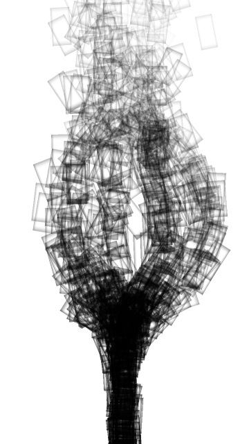
Let’s turn now to some of the rendering issues involved. Let’s assume you’ve got very little horsepower, or you’re working in a very small time slice — this might be why you’re using a noise-based solution anyway. You might only be capable of a one-thousand particle system instead of a one-million particle system. For your particles to be space-filling, consider adding some motion blur.

Motion blur might seem overkill at first, but since it inflates your billboards in an intelligent way, you can have fewer particles in your system. The image to the right (click to enlarge) shows how billboards can be stretched and oriented according to their velocities.

Note that it can be tricky to perform velocity alignment and still allow for certain viewing angles. For more on the subject (and some code), see this section of my previous blog entry.

Soft Particles

Another rendering issue that can crop up are hard edges. This occurs when you’re depth-testing billboards against obstacles in your scene — the effect is shown on the left in the image below.

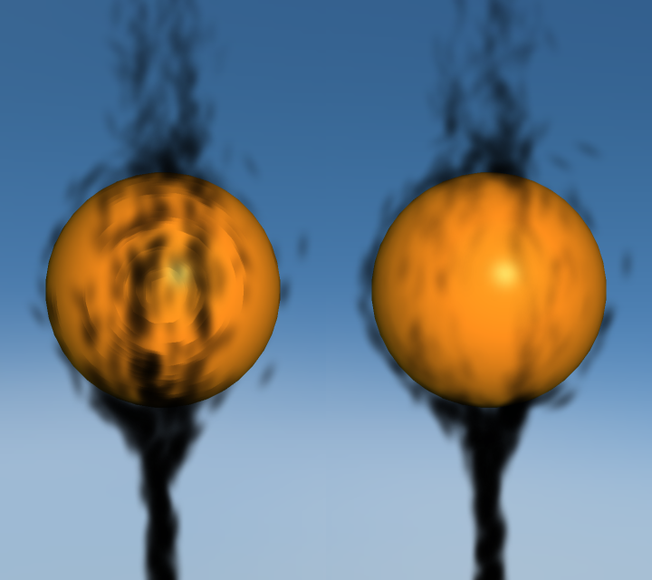
Turns out that an excellent chapter in GPU Gems 3 discusses this issue. (Here’s a link to the online version of the chapter.) The basic idea is to fade alpha in your fragment shader according to the Z distance between the current fragment and the depth obstacle. This method is called soft particles, and you can see the result on the right in the comparison image.

I found that using a linear fade-out can cause particles to appear too light. To alleviate this, I decided to apply a quartic falloff to the alpha value. This makes the particle stay opaque longer with rapid fall-off. When I’m prototyping simple functions like this, I like to use Wolfram Alpha as my web-based graphing calculator . Here’s one possibility (click to view in Wolfram Alpha):

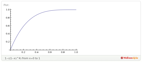
It’s tempting to use trig functions when designing ramp functions like this, but keep in mind that they can be quite costly.

Without further ado, here’s the fragment shader that I used to render my smoke particles:

uniform vec4 Color;
uniform vec2 InverseSize;
varying float gAlpha;
varying vec2 gTexCoord;
uniform sampler2D SpriteSampler;
uniform sampler2D DepthSampler;

void main()
{
    vec2 tc = gl_FragCoord.xy * InverseSize;
    float depth = texture2D(DepthSampler, tc).r;
    if (depth < gl_FragCoord.z)
        discard;

    float d = depth - gl_FragCoord.z;
    float softness = 1.0 - min(1.0, 40.0 * d);
    softness *= softness;
    softness = 1.0 - softness * softness;

    float A = gAlpha * texture2D(SpriteSampler, gTexCoord).a;
    gl_FragColor = Color * vec4(1, 1, 1, A * softness);
}

There are actually three alpha values involved in the above snippet: alpha due to the particle’s lifetime (gAlpha), alpha due to the circular nature of the sprite (SpriteSampler), and alpha due to the proximity of the nearest depth boundary (softness).

If you’d like, you can avoid the SpriteSampler lookup by evaluating the Gaussian function in the shader; I took that approach in my previous blog entry.

Next up is the compositing fragment shader that I used to blend the particle billboards against the scene. When this shader is active, the app is drawing a full-screen quad.

varying vec2 vTexCoord;
uniform sampler2D BackgroundSampler;
uniform sampler2D ParticlesSampler;

void main()
{
    vec4 dest = texture2D(BackgroundSampler, vTexCoord);
    vec4 src = texture2D(ParticlesSampler, vTexCoord);
    gl_FragColor.rgb = src.rgb * a + dest.rgb * (1.0 - a);
    gl_FragColor.a = 1.0;
}

Here’s the blending function I use when drawing the particles:

glBlendFuncSeparate(GL_SRC_ALPHA, GL_ONE_MINUS_SRC_ALPHA, GL_ZERO, GL_ONE_MINUS_SRC_ALPHA);

The rationale for this is explained in the GPU gems chapter that I already mentioned.

Streamlines

Adding a streamline renderer to your app makes it easy to visualize turbulent effects. As seen in the video to the right, it’s also pretty fun to watch the streamlines grow. The easiest way to do this? Simply use very small billboards and remove the call to glClear! Well, you’ll probably still want to clear the surface at startup time, to prevent junk. Easy peasy!

Downloads

I’ve tested the code with Mac OS X and Windows with Visual Studio 2010. It uses CMake for the build system.

• CurlNoise.zip
• Shaders.glsl

I consider this code to be on the public domain. Enjoy!