Sympy Surfaces

The OpenGL and Python code used to generate these images lives in this github project.

One way to play with tessellation shaders in OpenGL is by evaluating various parametric functions on the GPU. You can find plenty of parametric equations on the web, but I thought it would be fun to derive some interesting equations from scratch using a symbolic math package.

I didn’t want to shell out the cash for Mathematica so I looked around for open source solutions and settled on SymPy. Overall it feels much less mature than commercial packages – I can hang or crash it pretty easily, especially when I call simplify. But, it has a nice Pythonic API.

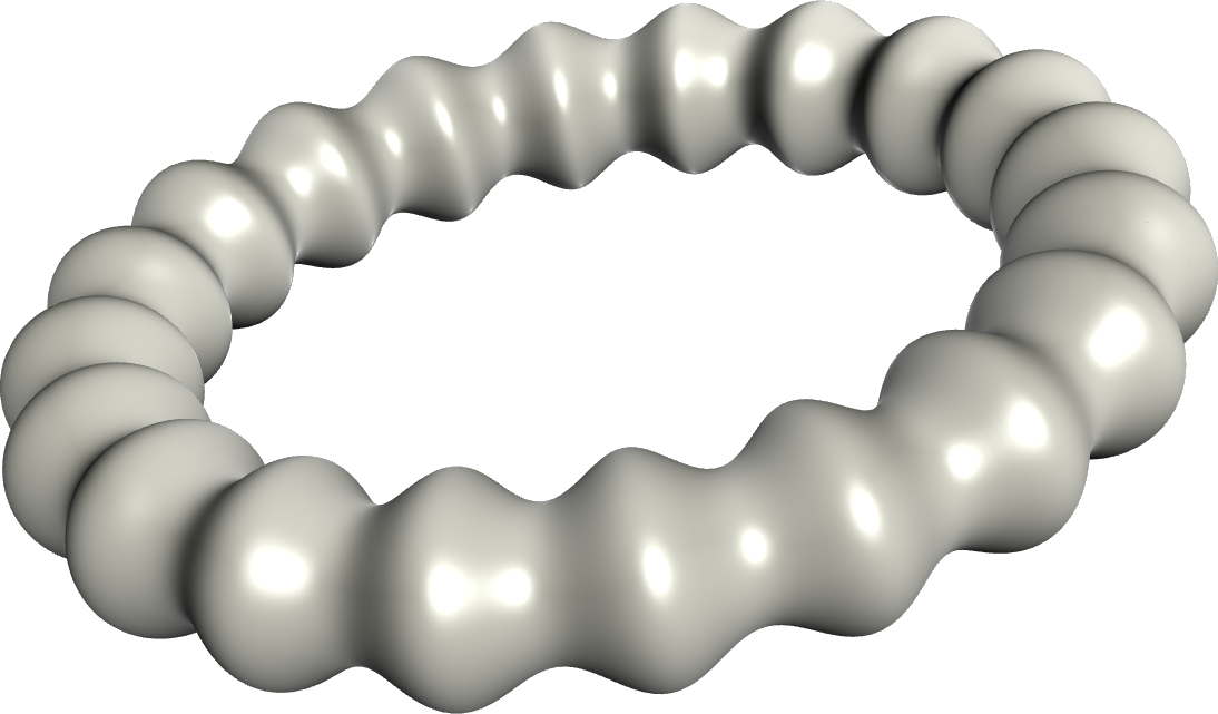
The parametric equation for a standard Torus is easy enough to find on the interwebs, but it’s a good starting point for our exercise. Let’s derive the parametric equation for a torus that has ridges, like this:

In SymPy, the Matrix class is an all-encompassing class that can represent matrices, vectors, and vector-valued functions. I found it convenient to create some helper functions with terse names:

from sympy.matrices import *

def VVF(*args):
    """Quicky construct a vector-valued function"""
    return Matrix(args)

def DVVF(m, variable):
    """Find a partial derivative of a vector-valued function"""
    return m.applyfunc(lambda f: diff(f,variable))

def PrintVVF(label, vvf):
    """ Print a vector-valued function using C syntax """
    print '// ' + label
    print "float x =", ccode(vvf[0]) + ";"
    print "float y =", ccode(vvf[1]) + ";"
    print "float z =", ccode(vvf[2]) + ";"

One advantage of deriving the torus equation from scratch is that we can easily come up with an analytic solution for computing the normal vector at an arbitrary point:

def NormalFunc(f):
    """Takes a vector-valued function of u and v"""
    """Computes formula for determining the surface normal at any point"""
    dfdu = DVVF(f, u)
    dfdv = DVVF(f, v)
    return dfdu.cross(dfdv)

To compute the parametric equation of a torus, we need a general way to sweep a circle along an arbitrary curve. We can use the Gram-Schmidt orthogonalization to formulate the Frenet frame:

u, v = symbols('u v', positive=True)

def Sweep(sweepCurve, crossSection):
    """ Takes two vector-valued functions:        """
    """ - sweepCurve is a function of u           """
    """ - crossSection is a function of v         """
    """ Returns a new vector-valued function      """
    """ that represents the composition of these. """
    # Compute first-order and second-order derivatives:
    d = DVVF(sweepCurve,u)
    dd = DVVF(d,u)
    # Perform Gram-Schmidt orthogonalization:
    t = d
    n = dd - t * dd.dot(t)
    b = t.cross(n).transpose()
    # Formulate the Frenet Frame:
    curveBasis = t.row_join(n).row_join(b)
    # Transform the cross section to the curve's space:
    s = sweepCurve + curveBasis * crossSection
    return s

We can now easily the derive the parametric equation for the ridged torus. The sweep curve is just a circle with radius R, and the cross section is a circle with radius r. To achieve the ridges, we’ll deform r using a sine wave:

# Vector-valued function that draws a circle on the Y-Z plane.
def CircleYZ(radius):
    return VVF(0, -radius*cos(v), radius*sin(v))

# Derive the formula for a ridged torus:
r, R = symbols('r R', positive=True)
h, f = symbols('h f')
sweepCurve = VVF(R*cos(u), R*sin(u), 0)
crossSection = CircleYZ(r + h*sin(u*f))
surface = Sweep(sweepCurve, crossSection)
normals = NormalFunc(surface)
PrintVVF('Ridged Torus Surface', surface)
PrintVVF('Ridged Torus Normals', normals)

The output should look something like this:

// Ridged Torus Surface
float x = R*cos(u) + (h*sin(f*u) + r)*cos(u)*cos(v);
float y = R*sin(u) + (h*sin(f*u) + r)*sin(u)*cos(v);
float z = (h*sin(f*u) + r)*sin(v);

// Ridged Torus Normals
float x = -f*h*(h*sin(f*u) + r)*sin(u)*pow(cos(v), 2)*cos(f*u) + f*h*(h*sin(f*u) + r)*sin(u)*cos(f*u) + (h*sin(f*u) + r)*(R*cos(u) + f*h*sin(u)*cos(v)*cos(f*u) + (h*sin(f*u) + r)*cos(u)*cos(v))*cos(v);
float y = f*h*(h*sin(f*u) + r)*cos(u)*pow(cos(v), 2)*cos(f*u) - f*h*(h*sin(f*u) + r)*cos(u)*cos(f*u) + (-h*sin(f*u) - r)*(-R*sin(u) + f*h*cos(u)*cos(v)*cos(f*u) + (-h*sin(f*u) - r)*sin(u)*cos(v))*cos(v);
float z = (-h*sin(f*u) - r)*(-R*sin(u) + f*h*cos(u)*cos(v)*cos(f*u) + (-h*sin(f*u) - r)*sin(u)*cos(v))*sin(u)*sin(v) + (h*sin(f*u) + r)*(R*cos(u) + f*h*sin(u)*cos(v)*cos(f*u) + (h*sin(f*u) + r)*cos(u)*cos(v))*sin(v)*cos(u);

The equation for the surface itself isn’t a surpising result, but it’s pretty cool to see an analytic solution for the normal vectors as well!

Superellipse Cross Section

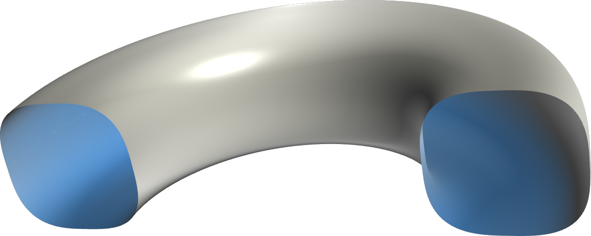
For the cross-section curve, let’s try something more interesting than a circle. How about a superellipse:

Since this “squircle torus” is just another swept surface, it’s just as easy to derive as the ridged torus:

# Vector-valued function that draws a superellipse on the Y-Z plane.
def SuperellipseYZ(n, a, b):
    x = (Abs(cos(v)) ** (2/n)) * a * sign(cos(v))
    y = (Abs(sin(v)) ** (2/n)) * b * sign(sin(v))
    return VVF(0, -x, y)

# Derive the formula for a squircle torus:
r, R = symbols('r R', positive=True)
n = symbols('n')
sweepCurve = VVF(R*cos(u), R*sin(u), 0)
crossSection = SuperellipseYZ(n, 0.5, 0.5)
surface = Sweep(sweepCurve, crossSection)
normals = NormalFunc(surface)
PrintVVF('Superellipse Torus Surface', surface)
PrintVVF('Superellipse Torus Normals', normals)

The resulting formulae are reasonably-sized:

// Superellipse Torus Surface
float x = (R - pow(cos(v), 2)*sign(cos(v))/4)*cos(u);
float y = (R - pow(cos(v), 2)*sign(cos(v))/4)*sin(u);
float z = pow(sin(v), 2)*sign(sin(v))/4;

// Superellipse Torus Normals
float x = (R/2 - pow(cos(v), 2)*sign(cos(v))/8)*sin(v)*cos(u)*cos(v)*sign(sin(v));
float y = (R/2 - pow(cos(v), 2)*sign(cos(v))/8)*sin(u)*sin(v)*cos(v)*sign(sin(v));
float z = (-R/2 + pow(cos(v), 2)*sign(cos(v))/8)*sin(v)*cos(v)*sign(cos(v));

Möbius Tube

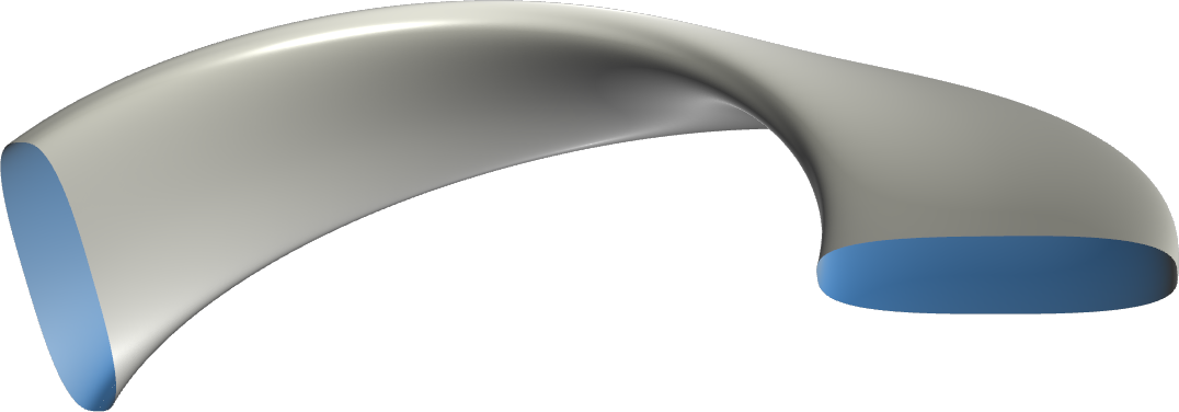
If we squish the superellipse and gradually rotate it, we can generate a nice Möbius Tube. Here’s the result, cut in half for clarity:

We can re-use our existing SuperellipseYZ function and add a rotation function to make this easier. Here’s one way of doing it:

# Rotates the given vector-valued function along the X-axis
def RotateX(f, q):
    y = f[1] * cos(q) - f[2] * sin(q)
    z = f[1] * sin(q) + f[2] * cos(q)
    x = f[0]
    return VVF(x, y, z)

sweepCurve = VVF(R*cos(u), R*sin(u), 0)
n = symbols('n')
crossSection = SuperellipseYZ(n, 0.5, 0.125)
crossSection = RotateX(crossSection, u / 2)
surface = Sweep(sweepCurve, crossSection)
PrintVVF('Superellipse Mobius Surface', surface)

And, here’s the result:

// Superellipse Mobius Surface
float x = R*cos(u) - (-0.0625*pow(sin(v), 2)*sin(2*v)*sign(sin(v)) + pow(cos(v), 2)*cos(2*v)*sign(cos(v))/4)*cos(u);
float y = R*sin(u) - (-0.0625*pow(sin(v), 2)*sin(2*v)*sign(sin(v)) + pow(cos(v), 2)*cos(2*v)*sign(cos(v))/4)*sin(u);
float z = (0.0625*pow(sin(v), 2)*cos(2*v)*sign(sin(v)) + sin(2*v)*pow(cos(v), 2)*sign(cos(v))/4)*(pow(sin(u), 2) + pow(cos(u), 2));

SymPy had trouble computing the partial derivatives in this case. Unfortunately, I found it pretty easy to run against its limitations, especially when I tried complex sweep curves.

It’s okay that we weren’t able to compute a one-shot formula for the Mobius tube’s normals, because the shader can use forward differencing, as we’ll see in the next section.

Rendering With Zero Vertex Attributes

If you’re using core profile, you can render one of these surfaces using one small patch, and no enabled vertex attributes whatsoever. Just make sure that you’re not using VAO zero. For example, on the C side:

glPatchParameteri(GL_PATCH_VERTICES, 4);
glDrawArrays(GL_PATCHES, 0, 4);

And, on the GLSL side:

-- Vertex Shader

void main() {}

-- Tess Control Shader

layout(vertices = 4) out;
void main() {
    gl_TessLevelInner[0] = gl_TessLevelInner[1] =
    gl_TessLevelOuter[0] = gl_TessLevelOuter[1] = 
    gl_TessLevelOuter[2] = gl_TessLevelOuter[3] = 128;
}

-- Tess Eval Shader

layout(quads, equal_spacing, ccw) in;

out vec3 tePosition;
out vec3 teNormal;
uniform mat4 Projection;
uniform mat4 Modelview;

subroutine vec3 ParametricFunction(float u, float v);
subroutine uniform ParametricFunction SurfaceFunc;

void main() {
    vec2 p = gl_TessCoord.xy * 2 * Pi;
    tePosition = SurfaceFunc(p.x, p.y);
    gl_Position = Projection * Modelview * vec4(tePosition, 1);
    
    // Use forward differencing to compute the normal:
    float du = 0.0001; float dv = 0.0001;
    vec3 C = SurfaceFunc(p.x + du, p.y);
    vec3 B = SurfaceFunc(p.x, p.y + dv);
    vec3 A = tePosition;
    teNormal = normalize(cross(C - A, B - A));
}

I left out the geometry shader and fragment shader since they’re pretty standard. The full blown code used to generate these images can be found in my github project. Enjoy!