Closest Point Coordinate Fields

This post introduces closest point coordinate fields (CPCF’s), which are two-channel images related to Voronoi diagrams and distance fields.

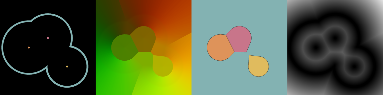
The image in the far left panel is an example seed image and its CPCF is depicted to its right. The CPCF was easily transformed into the Voronoi diagram and distance field shown in the two rightmost panels.

The Euclidean distance transform (EDT) can be defined as the following function, which consumes a set of seed points $𝒮$ and produces a value for every $p$ in $ℝ^{2}$ :

d (p) = \min_{q \in 𝒮} ∥p - q∥

Sampling the above function over a grid results in an unsigned distance field. (As opposed to a signed distance field, which can be generated via composition with an EDT that takes the complement of $𝒮$ .)

Felzenszwalb and Huttenlocher generalized this into the following equation, which is easiest to understand when considering a function $f$ that returns 0 if its input is in $𝒮$ , and ∞ otherwise.

d (p) = \min_{q \in ℝ^{2}} (∥p - q∥ + f (q))

This led to their linear-time algorithm, which is probably the best way to generate the SDF on a CPU, because it’s simple and fast.

Next I’d like to introduce a new function that leverages the EDT function, but produces a set of points instead of a scalar value:

g (p) = {q \in 𝒮 | ∥p - q∥ = d (p)}

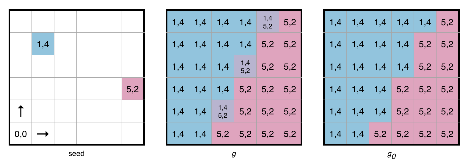
The above function usually results in a set that has only one element. The set has multiple items only when several seed points “tie for first place”, which occurs along the edges of the Voronoi diagram produced by $𝒮$ .

Let’s just pick a random tiebreaker from each set; we’ll call this $g_{0}$ instead of $g$ . If we sample $g_{0}$ over a grid, the result is the CPCF.

Typically you can accurately represent a CPCF using an image format that has two 16-bit integers per pixel.

The CPCF is cool because it can be trivially transformed into a distance field, but encodes more information than a distance field.

CPCF’s are the direct result of Rong and Tan’s jump flooding algorithm, which is probably the fastest way to compute a distance field on a GPU.

Here’s how to transform a CPCF into a distance field:

d (p) = ∥p - g_{0} (p)∥

In GLSL, transforming a CPCF into a distance field looks like this:

dist = distance(uv, texture(cpcf, uv).st);
gl_FragColor = vec4(dist, dist, dist, 1);

Drawing a Voronoi diagram can be accomplished by sampling from the CPCF and the seed image:

vec2 st = texture(cpcf, uv).st;
gl_FragColor = texture(seed, st);

Applications

Warped CPCF’s

In the following image sequence, we apply a warping operation to the CPCF using several octaves of Perlin noise. The resulting Voronoi diagram is terrain-like, with interesting political boundaries. In the last panel, we use the implicit distance field to create mountains and radiating contours.

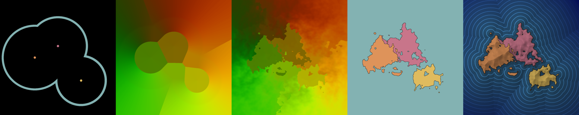
These images were generated using the archipelago functionality (doc page) in the heman C library (github project).

Closest Point Picking

DistancePicking Screenshot

Another use of CPCF’s is fuzzy picking. With modern GPU’s, you can continuously perform jump flooding on a low-resolution framebuffer in real time. By making an O(1) lookup into the resulting CPCF, you can obtain the nearest “pixel of interest” relative to the user’s touch point.

High Quality Magnification

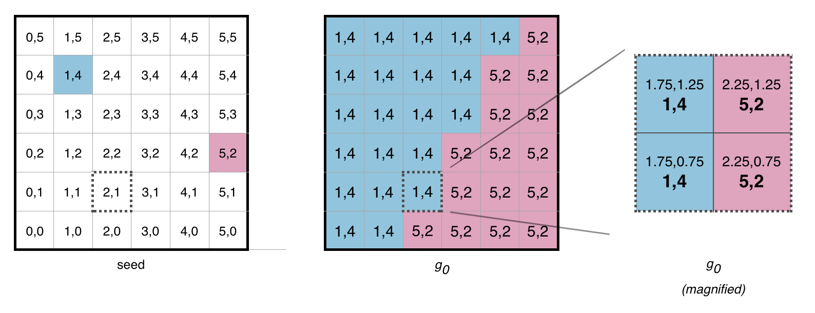
Coordinate fields enable high quality magnification of Voronoi diagrams using only image data. The following diagram illustrates 2x magnification of the CPCF pixel at 2,1, which happens to be equidistant from the two seed points. In the middle panel, we arbitrarily chose the blue seed as the tiebreaker. In the far right panel, we’ve computed 4 new CPCF values. Each new value is computed by sampling 4 pixels from the middle panel, reevaluating the distances to their referenced seed points, and selecting the minimum values.

Philip Rideout
October 2015

Coffee should be hot as hell, black as the devil, pure as an angel, sweet as love.