
Barnette’s Conjecture for Humans, Part 1
If you are familiar with my blog you know I’m a bit obsessed with the Graceful Tree Conjecture, but my second favorite graph theory conjecture is (was?) Barnette’s conjecture. It got promoted to a theorem in the 6-Oct-2026 Mathocalypse. In this post I’ll explain the conjecture, and, in part, the proof. I’ll finish my exposition of the proof in a follow-up post.
When I first flipped through the OpenAI proof, I thought, Hey, this looks reasonable, I should be able to handle it. It ended up taking me several weekends. The paper is strangely dense and has an awkward overall flow, and it has only one pathetic little figure, despite being a proof that lends itself to visuals. So I felt motivated to write this post.
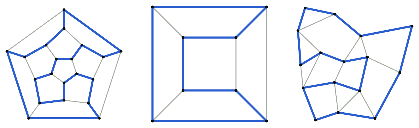
First, a quick refresher: a Hamiltonian cycle is a walk along the edges of a graph that visits every vertex exactly once and ends up back where it started. A graph that has one is Hamiltonian. Here are three Hamiltonian graphs, each with a Hamiltonian cycle in blue:
It’s a bit tricky to look at a graph and quickly determine if it is Hamiltonian, which makes it an interesting area of study. There are, however, a few well-known facts. For example, Dirac’s theorem says that a graph is Hamiltonian if every vertex has enough neighbors (see my previous post).
Outside of Dirac’s theorem and its descendants, there are disappointingly few easy-to-state theorems for recognizing Hamiltonian graphs. Here’s a famous exception:
Every 4-connected planar graph is Hamiltonian.
A graph is planar if you can draw it without any of its edges crossing, and it’s 4-connected if it stays connected after you remove any 3 of its vertices.
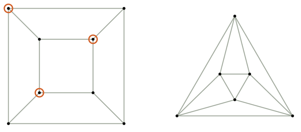
Likewise, a graph is 3-connected if it stays connected after you remove any 2 of its vertices. Every 4-connected graph is 3-connected, but not the other way around. In the following figure, the cube on the left is 3-connected but not 4-connected: remove the three circled vertices, and the vertex they surround is cut off from the rest. The octahedron on the right is 4-connected.
Barnette’s conjecture is exciting because it’s the same rare kind of statement as Tutte’s, and stood open for 57 years:
Every 3-connected planar graph that is cubic and bipartite is Hamiltonian.
A graph is cubic if every vertex has exactly three edges. It’s bipartite if you can color its vertices black and white, such that every edge joins a black vertex to a white one. A graph that’s 3-connected, planar, cubic, and bipartite is a Barnette graph.
There’s some drama behind that list of four properties. Leave out “bipartite” and you get Tait’s conjecture, from 1884, which would have proven the four color theorem if it were true. It stood for 62 years, until Tutte found a counterexample. Tutte then made a conjecture of his own, which leaves out “planar” instead, and by 1976 Horton had sunk that one with a counterexample. Barnette’s conjecture has both qualifiers and has stood the test of time.
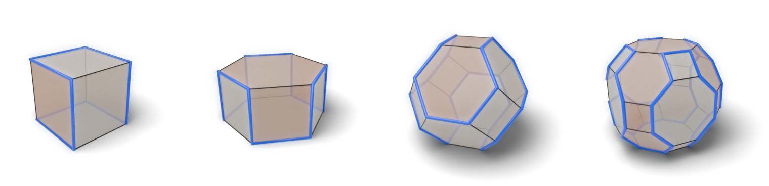
By the way, another way of saying 3-connected planar graph is “convex polyhedron” (Steinitz’s theorem). Here are four polyhedra, each with a Hamiltonian cycle in blue:
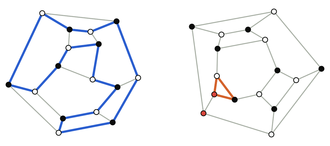
There’s another way to recognize a bipartite graph. Walk around a cycle in one and the two colors alternate. You arrive back where you started after an even number of steps, so every cycle must have even length, including the one around each face. In a planar graph, it works the other way too: if every face has an even number of sides, then the graph is bipartite.
In the following figure, the graph on the left is bipartite. The graph on the right isn’t: it has a face with three sides.
So, here’s another way of stating Barnette’s conjecture:
If a convex polyhedron has 3 edges at each corner, and every face has an even number of sides, then it must have a Hamiltonian cycle.
On the way to a proof, we’re going to reformulate the conjecture yet again, but first let’s take a step back and gaze upon the overall proof strategy:
This post will cover everything in the above chart except the Prime branch, which is where the juicy new stuff lives, so we’ll defer it to Part 2.
You might be wondering what a “harlequin” is; we’ll cover that later in this post. It’s just some made-up terminology that I think makes the proof easier to digest, especially in Part 2.
1. Dual reformulation
We’ve already restated the conjecture once, now let’s do it again by examining the dual of a Barnette graph (put a vertex in each face, and join two vertices whenever their faces share an edge).
Before taking a dual, let’s see what a Hamiltonian cycle does to the faces of a polyhedron. Take the truncated octahedron from earlier. Its Hamiltonian cycle is a closed loop, so it cuts the surface of the polyhedron into two pieces. Drag the slider under the following video to cut it open.
On the left of the next figure, the same polyhedron is flattened, with the faces inside its cycle tinted. Drag the slider to stretch the inside and outside into round disks, with the cycle around each rim.
Every vertex lies on the cycle, and the graph is cubic, so every vertex has exactly one edge that isn’t part of the cycle. Those leftover edges are chords. Two chords never cross, because planar drawings do not have crossings. The region around the outside of the flat drawing is also a face, and it ends up in the middle of the right disk.
Now put a vertex in each face of a disk, and join two vertices whenever their faces share a chord. Every chord cuts its disk in two, so there’s exactly one route from any face to any other. That makes both of these graphs trees, which are connected graphs that have no cycles.
The dual of any cubic planar graph is a triangulation. Below are two triangulations, which are duals of Barnette graphs. Each is depicted with a blue Hamiltonian cycle from its source graph, and the two trees resulting from the cut.
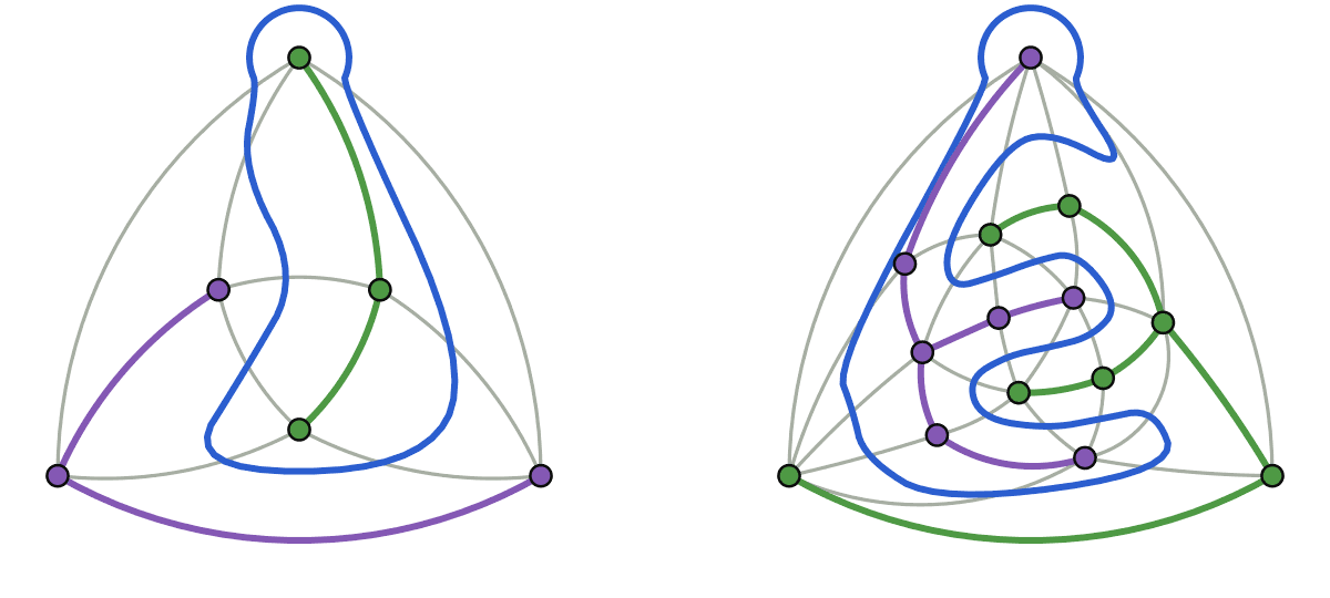
So a Hamiltonian cycle makes two trees. It works the other way, too:
A cubic polyhedral graph has a Hamiltonian cycle if and only if you can color the vertices of its dual triangulation green and purple, such that each color induces a tree.
Sherman Stein proved this at UC Davis, a couple of years after his colleague David Barnette made his conjecture. We’ve already seen how the easy direction works, from a Hamiltonian cycle to two trees. The other direction is a bit trickier, but Stein proved it too.
That gives us Barnette’s conjecture in terms of the dual: the vertices of the dual of every Barnette graph can be colored green and purple, such that each color induces a tree.
Nothing so far is new, but it’s all necessary to understand the OpenAI proof.
2. Harlequins and root triangles
The face-colored dual of a Barnette graph is so central to the proof that it deserves a name:
A harlequin is a polyhedron whose faces are all triangles, colored black and white so that every edge has a black triangle on one side and a white one on the other.
Every harlequin is the dual of a Barnette graph, and vice versa. Here are the earlier four polyhedra again, with their corners colored black and white. Under each one is its dual harlequin, first in 3D, then flat.
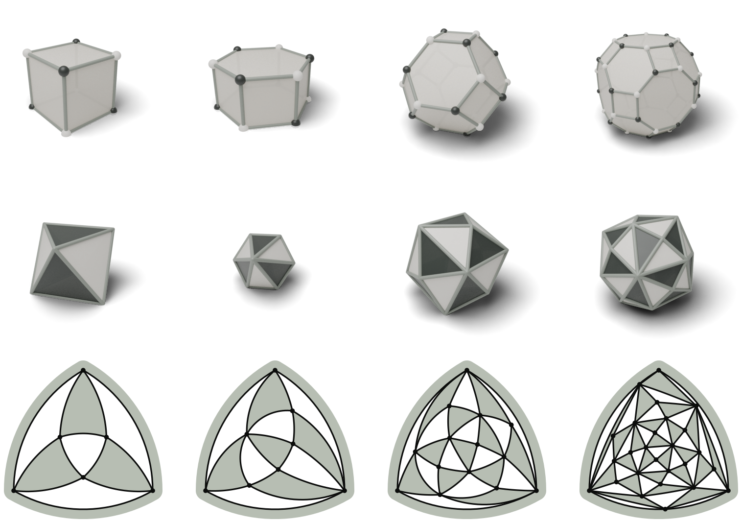
Every harlequin can be flattened the same way: pick a black triangle, poke a hole in it, and stretch it out. The gray band around each of the above 2D drawings is the black triangle with the hole, which now goes around the outside.
Let’s call that black triangle the root triangle. Any black triangle can be the root triangle.
The harlequin colors aren’t decoration, by the way. They’re the “bipartite” in Barnette’s conjecture. This post uses those colors only once, when we cut a harlequin in two, but Part 2 leans on them constantly.
3. Strengthening the conjecture
In 1986, the Soviet mathematician Alexander Kelmans showed that Barnette’s conjecture is equivalent to something stronger: every edge of every Barnette graph is skipped by some Hamiltonian cycle.
For example, take the cube. Here are all six of its Hamiltonian cycles:

Pick any edge, and in at least one drawing, it’s gray.
A Hamiltonian cycle skips an edge exactly when the edge of the harlequin that crosses it is in one of the two trees. You can see this in the two triangulations from earlier, where the blue loops never cross a green or purple edge. If we combine Kelmans’s theorem with Stein’s, in our harlequin language, we get:
For every harlequin
Not just any pair of trees will do, though. The following figure shows a harlequin colored two ways, each from a Hamiltonian cycle of its dual. On the left, the edge
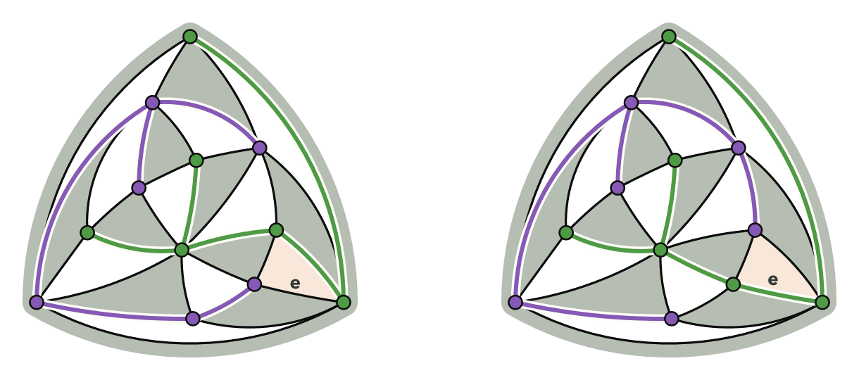
So the coloring on the left is not the kind that the conjecture asks for, at least not for this edge
4. Separating triangles
A separating triangle is a 3-cycle that is not a face. In the following figure, the harlequin on the left has no separating triangle: every loop of three edges is the outline of a face, even the one around the outside, which is the root triangle. The other two each have a separating triangle, in orange, with vertices both inside and outside of it.
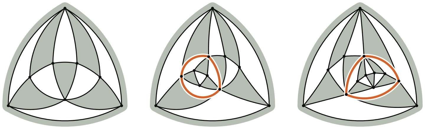
The proof of the harlequin version of Barnette’s conjecture splits into two cases, depending on whether a harlequin has a separating triangle. A harlequin that has one is composite, and a harlequin that doesn’t is prime.
A separating triangle cuts the harlequin in two, with vertices on both sides, so a composite harlequin comes apart into two smaller pieces.
5. Composite harlequins: proof by induction
Let’s check where we are in the flow chart. We’re trying to prove the harlequin version of Barnette’s conjecture: for every edge
Cut a composite harlequin
The plan is to cut
Cutting a Barnette graph this way is an old trick: Holton, Manvel, and McKay did it in 1985.
Here’s an illustration of a composite harlequin being cut into two smaller harlequins:
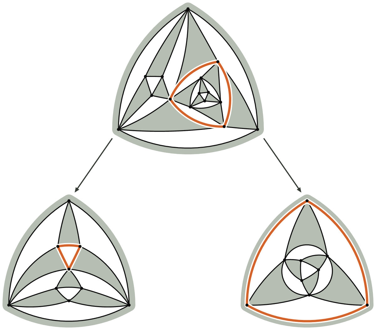
First, a fact about colors: the three triangles just outside a separating triangle always have the same color, and the three just inside have the other color. This is a known result, and can be proven with a simple counting argument.
Which color ends up outside depends on where the root triangle is. Any black triangle can be the root. From here on, we’ll always pick the root so that the three triangles just outside the separating triangle are black, like in the figure above.
Cutting along the separating triangle gives
- The outer child keeps everything outside the separating triangle.
- The inner child keeps everything inside the separating triangle.
Either way, the cut leaves a hole with three edges around it, and one new triangle fills the hole:
Let
Both patches are outlined in orange above. The outer child’s patch is the small triangle in the middle of its drawing. The inner child’s patch goes around the outside of its drawing, which makes it the root triangle.
The outer child’s patch borders the three black triangles just outside the separating triangle, so it’s white. The inner child’s patch borders the three white triangles just inside, so it’s black, which is just what a root triangle should be. Every edge still straddles a black triangle and a white one. That makes both children harlequins.
Color each child’s vertices green and purple, so that each color induces a tree:
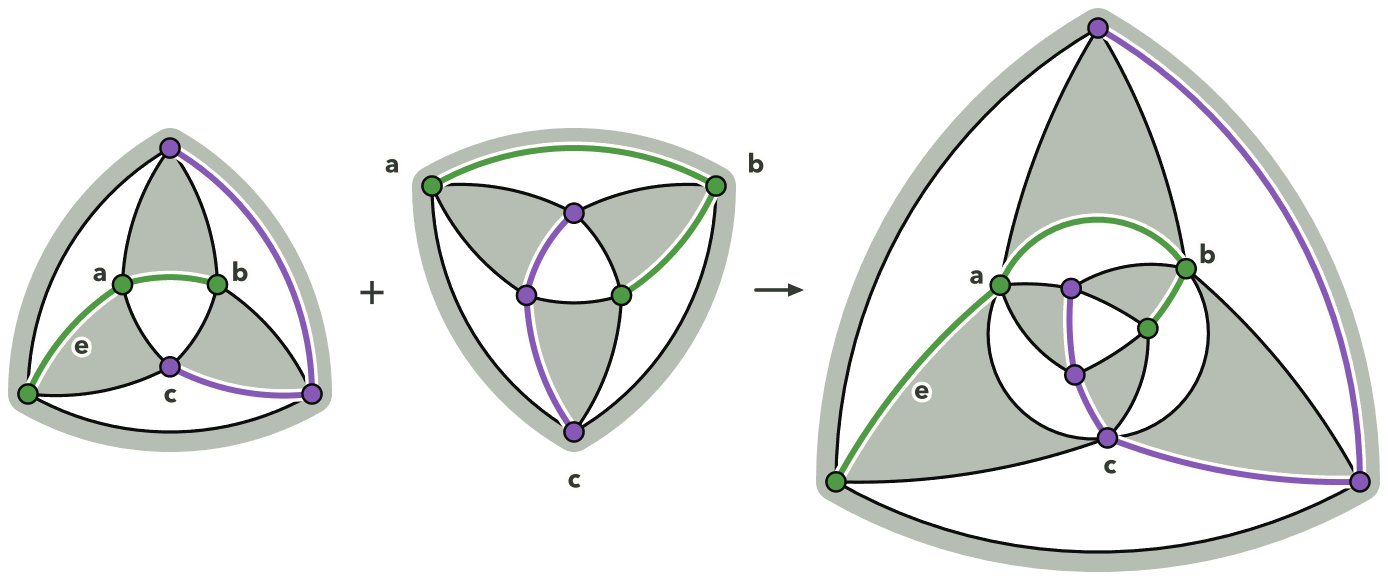
Exactly one side of every triangle is in a tree, since its three corners can’t all share a color, or they’d make a cycle. That includes each child’s patch.
On the left of the above figure is the outer child, colored so that the edge
In the middle drawing is the inner child, where
Then glue them, as in the right drawing. The purple trees meet only at
That sets up an induction on the number of vertices. Suppose that every prime harlequin can be colored like that, for each of its edges. Then every composite harlequin can too: cut it in two, color its children by induction, and glue.
So now the harlequin version of Barnette’s conjecture comes down to the prime harlequins, and that’s what Part 2 of this post will be all about. Stay tuned!
6. References
- The OpenAI proof: Paired states and Hamiltonian cycles in cubic bipartite planar graphs, 2026.
- David Barnette’s conjecture: Conjecture 5, page 343 of Recent Progress in Combinatorics, edited by W. T. Tutte, 1969.
- W. T. Tutte, A theorem on planar graphs, Transactions of the American Mathematical Society, 1956. Tutte’s theorem.
- Sherman Stein, B-sets and planar maps, Pacific Journal of Mathematics, 1971. The green and purple trees.
- Alexander Kelmans, Constructions of cubic bipartite 3-connected graphs without Hamiltonian cycles, American Mathematical Society Translations, Series 2, volume 158, 1994 (the Russian original is from 1986). The strengthening. It isn’t free to read, but Alexander Hertel’s A survey & strengthening of Barnette’s conjecture (2005) states it as Theorem 10.
- Derek Holton, Bennet Manvel, and Brendan McKay, Hamiltonian cycles in cubic 3-connected bipartite planar graphs, Journal of Combinatorial Theory, Series B, 1985. Cutting and gluing along a separating triangle.
- Maximilian Gorsky, Raphael Steiner, and Sebastian Wiederrecht, Matching theory and Barnette’s conjecture, 2022. Lemma 4.5 is the induction for composite harlequins, in the dual.